Introduction to Convolutional NN

Design Goals

We want to be invariant to some transformations but also at the same time to be specific to some thing. Convolutional Neural Networks (CNNs) are a class of deep neural networks that are particularly effective for image processing tasks. They are designed to automatically and adaptively learn spatial hierarchies of features from images. Compared to standard Fully connected Neural Networks, they reuse weights, making their number of parameter much fewer.

Historically, they were inspired by the visual cortex of animals, where simple cells respond to specific orientations and complex cells respond to combinations of simple cells. See Hubel and Wiesel experiment, they also saw that there is some hierarchical organization of how the cells communicate with each other.

The convolution operator

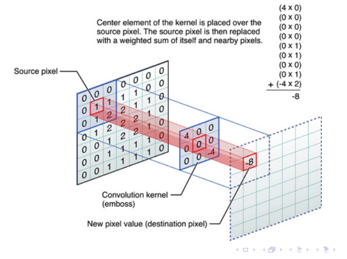
$$ \begin{align*} I'(i,j) &= \sum_{m=-k}^{k} \sum_{n=-k}^{k} I(i - m, j - n) K(m, n) \\ &= \sum_{m=-k}^{k} \sum_{n=-k}^{k} I(i + m, j + n) K(-m, -n) \end{align*} $$

Il prodotto di convoluzione è matematicamente molto contorto, anche se nella pratica è una cosa molto molto semplice. In pratica voglio calcolare il valore di un pixel in funzione di certi suoi vicini, moltiplicati per un filter che in pratica è una matrice di pesi, che definisce un pattern lineare a cui sarei interessato di cercare nell’immagine.

Shift-Equivariance Property

$$ (\mathcal{T \circ \text{ shift }})(g) = (\text{shift} \circ \mathcal{T})(g) $$

Correlation operator

$$ (f*g)(t) = \sum_{\tau = -\infty}^{\infty} f(\tau)g(t-\tau) $$

Pytorch usually learns correlations, but calls it convolution, because the orientation of the filter is learned does not matter much. The two operations are equivalent given symmetric kernels.

$$ I'(i, j) = \sum_{m = -k}^{k} \sum_{n = -k}^{k} I(i + m, j + n) K(m, n) $$

With $k = \text{floor}\left( \frac{M}{2} \right)$ square kernel of size $M$.

• Slides ed esempi (molto più chiaril) Vedi che per calcolare quell’8 sto facendo cose lineari con tutti pixel intorno ad essa.

  

Questo operatore l’abbiamo già trattato in modo molto breve in Deblur di immagini.

Counting the parameters

• Convolutional layer
  • $C_{out} = \text{number of filters}$
  • $C_{in} = \text{number of channels}$
  • $K = \text{kernel size}$

The number of parameters is just dependent on the above three values, and the presence of the bias:

$$ \text{Num Params} = C_{out} \cdot (C_{in} \cdot K^{2} + 1) $$

Where $1$ is from the bias parameter.

Size of the output

The size of the output is given by the formula: $$ \begin{align*}

\text{Output Size} &= \left\lfloor \frac{L_{in} + 2P - D \cdot (K - 1) - 1}{S} + 1 \right\rfloor\ \end{align*} $$

Some properties and uses

Sappiamo tutti che le immagini non sono altro che arrai di valori in un certo intervallo, che rappresentano l’intensità dei colori, o solamente del bianco-grigio nel caso delle immagini grigio nere.

Queste intensità si potrebbero anche rappresentare come superfici 3d in cui la posizione del pixel identifica x e y, mentre l’intensità la z, abbiamo quindi proprio delle superfici!, delle montagne, valli fiumi etc. Le cose molto interessanti sono cambi di intensità improvvisi (con derivata molto alta) ossia i dirupi, le valli, questo cambio improvviso (il cambio di fase come dice Pedro di Master algorithm) è classico anche in nautura, è la parte con qualche informazione di interesse diciamo.

THE IDEA OF DERIVATIVE FOR CHANGES

• Slide finite approssimation of derivative

Comparison with Fully Connected

• Parameter sharing: convolutional networks share the parameters while fully connected do not.
• Local connectivity: in convolution layers neurons are connected only locally while in fully connected layers neurons are connected globally.

HMAX model

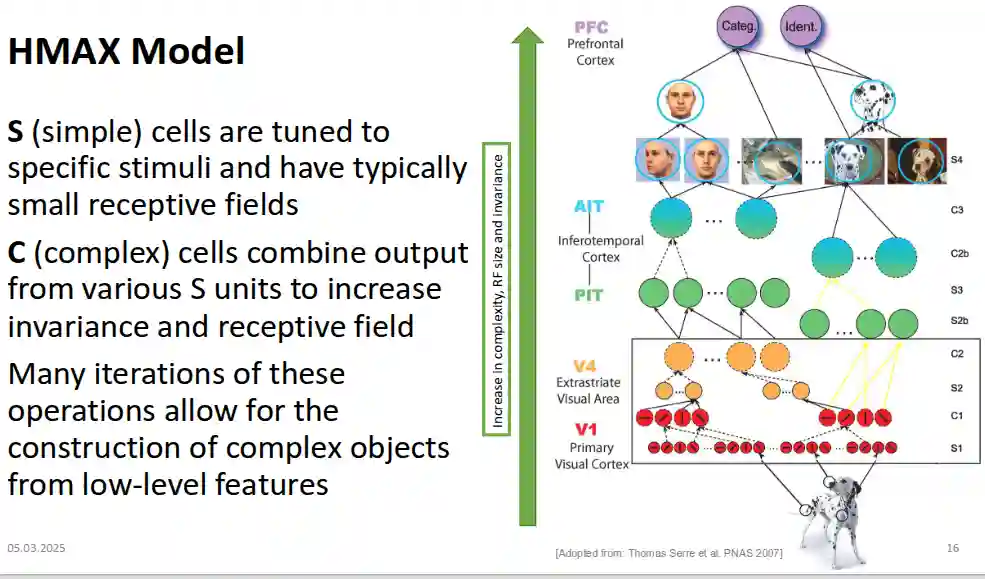
The fundamental principle of HMAX model is the hierarchy of cells that encode deeper and more complex features (higher receptive fields). HMAX is hierarchical and consists of alternating layers of:

1. Simple (S) units – increase selectivity (like feature detectors).
2. Complex (C) units – increase invariance (like pooling operations).

The $S$ cell is basically a gaussian. $w_{j}$ is some sort of parameter.

$$ y = \exp(- \frac{1}{2\sigma^{2}} \sum_{i} (x_{i} - w_{j})^{2}) $$$$ y_{j} = \max_{j = 1 \dots N} x_{j} $$

Trained with unsupervised learning.

Some what close to transfer learning: after you represented the lower features, you can use them for different tasks and just train the higher layers.

A brief history of CNNs

• Neurocognitron, mostly historical, but laying the groundwork for CNNs
• LeNet-5 one of the first dense nets, for handwritten digits
• Then you have AI winter until 2012 with AlexNet.

Image Filtering

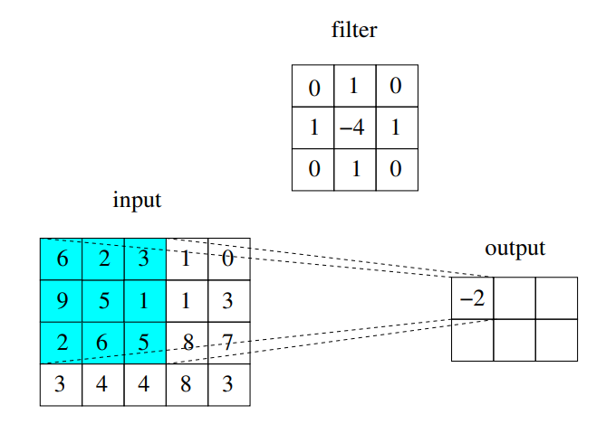
Image filtering modifies pixels in an image based on the values of neighboring pixels. The convolution operator is used to apply a filter (kernel) to an image, which can enhance or suppress certain features.

Usually they are linear transforms, see Spazi vettoriali

Visualization of Learned Features

We can recover the image that maximally activates some layer of neurons, from these images we see that convolutional networks are highly sensitive to some kinds of activations, and generally are able to recover complex shapes and patterns starting from those.

This actually helped to gain some insight to improve the performance of the network (they reduced the kernel size and went deeper, e.g. VGG model)

Some architectures

Deepwise separable convolution

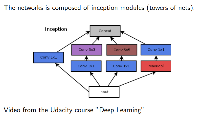
Inception architecture

Andiamo a derfinire un modulo di inception (in cui va a fare in un certo senso scrambling, decomporre e recomporre dati, in che modo vanno ad estrarre delle features io non lo so!).

Comunque questa è l’architettura classica, andare ad utilizzare reti convoluzionali e poi operarle con reti deep (alla fine non molto deep) in modo da collegargli insieme.

• Esempio di inception module Un esempio è GoogleLeNet (molte computazioni in parallelo)

https://www.youtube.com/watch?v=VxhSouuSZDY&ab_channel=Udacity

1x1 is to reduce the number of channels (way to reduce the parameter count) in the following layers! So that the number of input channels is ok.

Residual layers

Residual learning is the main concept of these networks, it’s when we have a direct link with the beginning! In pratica diamo la possibilità al neurone di scegliere di non modificare o invece sì l’input credo, provo a chiedermi se posso avere un valore migliore di quanto ho attualmente con qualche peso.

• Structure of residual layer (He et al. 2016).

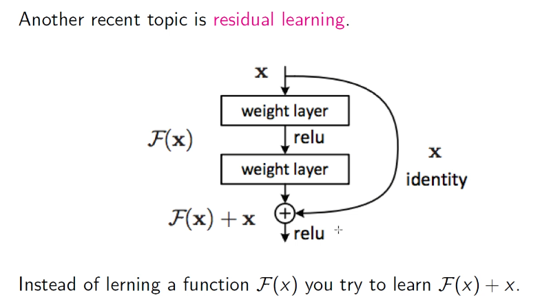
Usually these links help the network learn (lesser vanishing gradient.

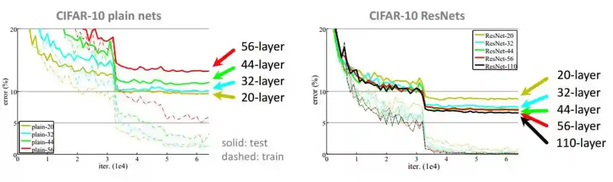
Shattered Gradients

Most gradient descent methods assume to have a smooth gradient. This is not true anymore with very deep layers. Adding residual layers help ease this problem. The residual error signal is actually necessary to train these networks, as the following images show.

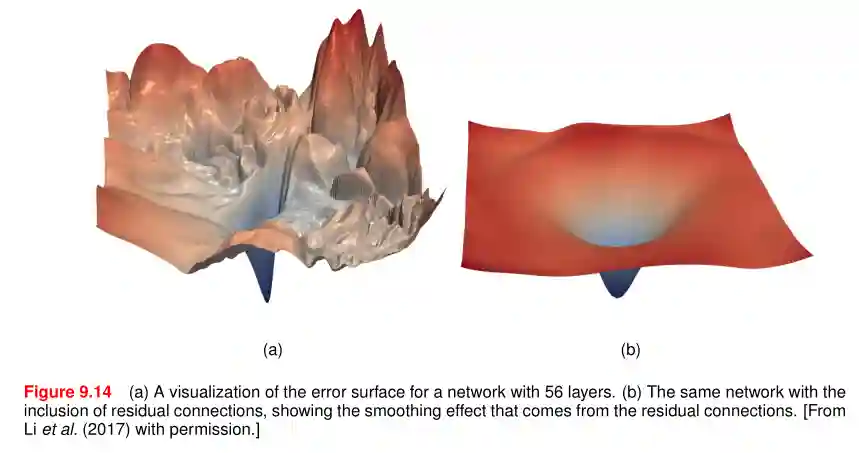
Smoother Error Surfaces

Introducing the residual layer helps in having smoother residual layers:

Residual Networks help gradient flow

In this section we provide a simple derivation of how residual layers help gradient flow.

$$ \begin{align*} h &= \sigma(Wx + b) \\ y &= Vh + c \end{align*} $$

Where:

• $x$ is the input.
• $W$ and $V$ are weight matrices.
• $b$ and $c$ are bias vectors.
• $\sigma$ is the activation function (like ReLU).

During back-propagation, we calculate the gradient of the loss ($L$) with respect to the input ($x$), denoted as $\frac{\partial L}{\partial x}$. Using the chain rule:

$$ \frac{\partial L}{\partial x} = \frac{\partial L}{\partial y} \cdot \frac{\partial y}{\partial h} \cdot \frac{\partial h}{\partial x} $$

Expanding this:

• $\frac{\partial y}{\partial h} = V^T$ (the transpose of the output layer weights)
• $\frac{\partial h}{\partial x} = \sigma'(Wx + b) \cdot W^T$ (the derivative of the activation function times the transpose of the input layer weights)

So, for the simple feed-forward network:

$\frac{\partial L}{\partial x} = \frac{\partial L}{\partial y} \cdot V^T \cdot \sigma'(Wx + b) \cdot W^T$

The Issue: If $\sigma'(Wx + b)$ (the derivative of the activation function) becomes very small (e.g., when sigmoid functions saturate or ReLU outputs are negative), this term can shrink the entire gradient. In deep networks, multiplying by such small terms repeatedly can cause the gradient to vanish to zero, stopping learning in early layers.

Now, let’s add a residual (or skip) connection. For a simple block, the output $y$ includes the original input $x$:

$h = \sigma(Wx + b)$ $y = h + x$

Again, we calculate $\frac{\partial L}{\partial x}$:

$\frac{\partial L}{\partial x} = \frac{\partial L}{\partial y} \cdot \frac{\partial y}{\partial x}$

Now, let’s find $\frac{\partial y}{\partial x}$:

$y = \sigma(Wx + b) + x$

Taking the derivative with respect to $x$:

$\frac{\partial y}{\partial x} = \frac{\partial (\sigma(Wx + b))}{\partial x} + \frac{\partial x}{\partial x}$ $\frac{\partial y}{\partial x} = \sigma'(Wx + b) \cdot W^T + I$ (where $I$ is the identity matrix, representing the derivative of $x$ with respect to $x$)

Substituting this back into the $\frac{\partial L}{\partial x}$ equation:

$$ \frac{\partial L}{\partial x} = \frac{\partial L}{\partial y} \cdot (\sigma'(Wx + b) \cdot W^T + I) $$$$ \begin{align*} \frac{\partial L}{\partial x} = \frac{\partial L}{\partial y} \cdot \sigma'(Wx + b) \cdot W^T + \frac{\partial L}{\partial y} \cdot I \end{align*} $$

The crucial part is the addition of the $\frac{\partial L}{\partial y}$ term in the residual network’s gradient.

• Direct Gradient Path: This $\frac{\partial L}{\partial y}$ term means that a portion of the gradient flows directly from the output $y$ back to the input $x$, unmodified by the weights or activation functions of the internal residual branch.
• Combating Vanishing Gradients: Even if the $\sigma'(Wx + b) \cdot W^T$ part (the “normal” gradient path) becomes very small, the $\frac{\partial L}{\partial y}$ term provides a guaranteed, direct path for the gradient. This ensures that earlier layers still receive substantial gradient updates, making it much easier to train very deep networks without the vanishing gradient problem.

In essence, the skip connection acts like a shortcut for gradients, allowing them to bypass layers where they might otherwise diminish, ensuring robust backpropagation through the entire network.

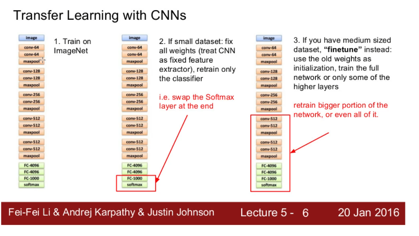
Transfer learning

• expected graph with performance with transfer learning

!

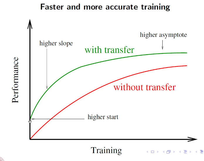
Comunque l’intuizione principale del transfer learning è l’idea che i primi layers facciano una sorta di estrazione di features più ad alto livello utili poi ai layers di deep NN. Se questa prima parte l’ho trainata su un corpus enorme, allora gli aspetti che è riuscito a generalizzare potrebbero essere utili anche per altro, e quindi utilizzo i pesi trovati in questa rete anche per altro, senza problemi.

Fine tune o finetuning è un pò rischioso, faccio un freeze di una parte del network più larga, potrei andare a overfittare e fare cose simili! Però ha più senso, ci aiuta a rendere l’intera architettura ancora più focussato in quello che vogliamo fare noi (in un certo senso forse dà via alcune generalizzazioni inutili nel nostro dominio)

Training of CNN

Backpropagation of CNNs

We can unroll the input and output layers as a single linear trasformation of a deep network (with weights adjusted accordingly).

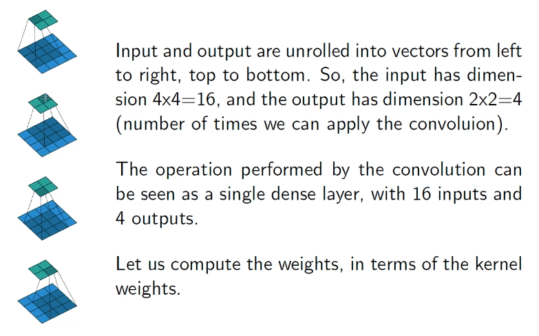
But how do we unroll?? We can see everything as a matrix with $[input\_size \times output\_size]$ as you can see from the image in the toggle

After we have modeled this matrix, we can learn using standard backpropagation we have talked about in Neural Networks.

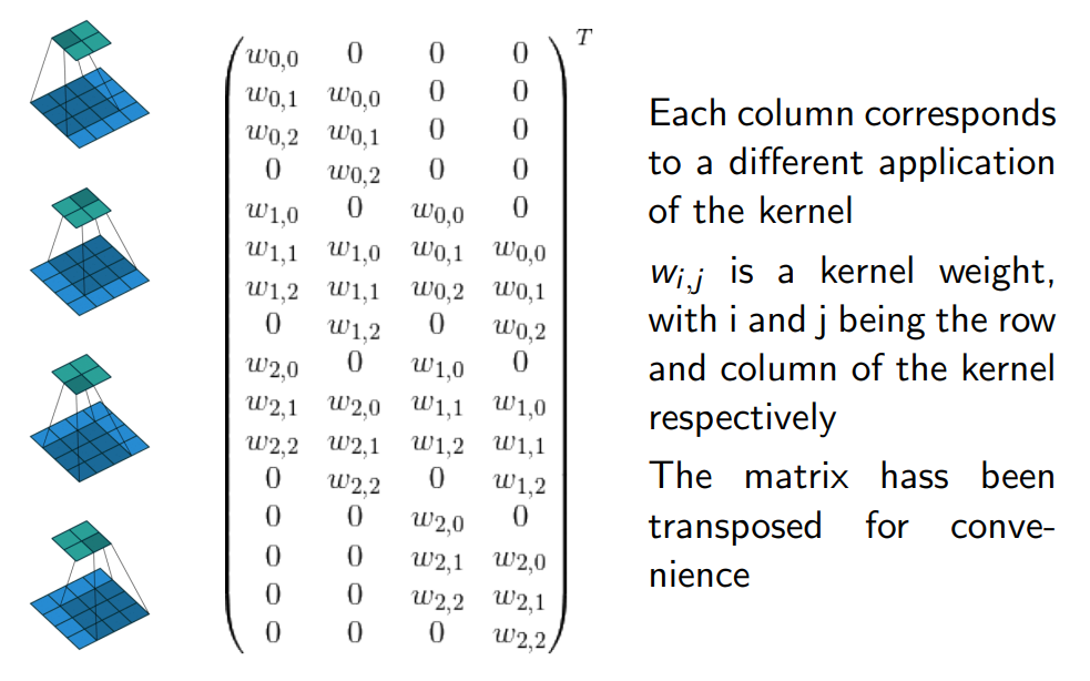
One problem with this method is that the matrix is sparse if the input is very large and the kernel is small. This would result in a very high number of zeros, making it not very efficient to store in this way.

Another aspect of this matrix is the shifted repetition of weights. These weights are the same in each column of the matrix, but simply shifted. This changes how weight updates are performed; a weighted average update is used.

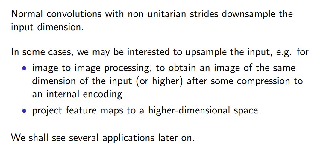
Transposed Convolutions

After too much downsampling with CNNs, I might want to increase the dimension again (for example, if the input is an image). Transposed convolutions allow us to increase the dimension back up. (I believe statistical techniques also work for this).

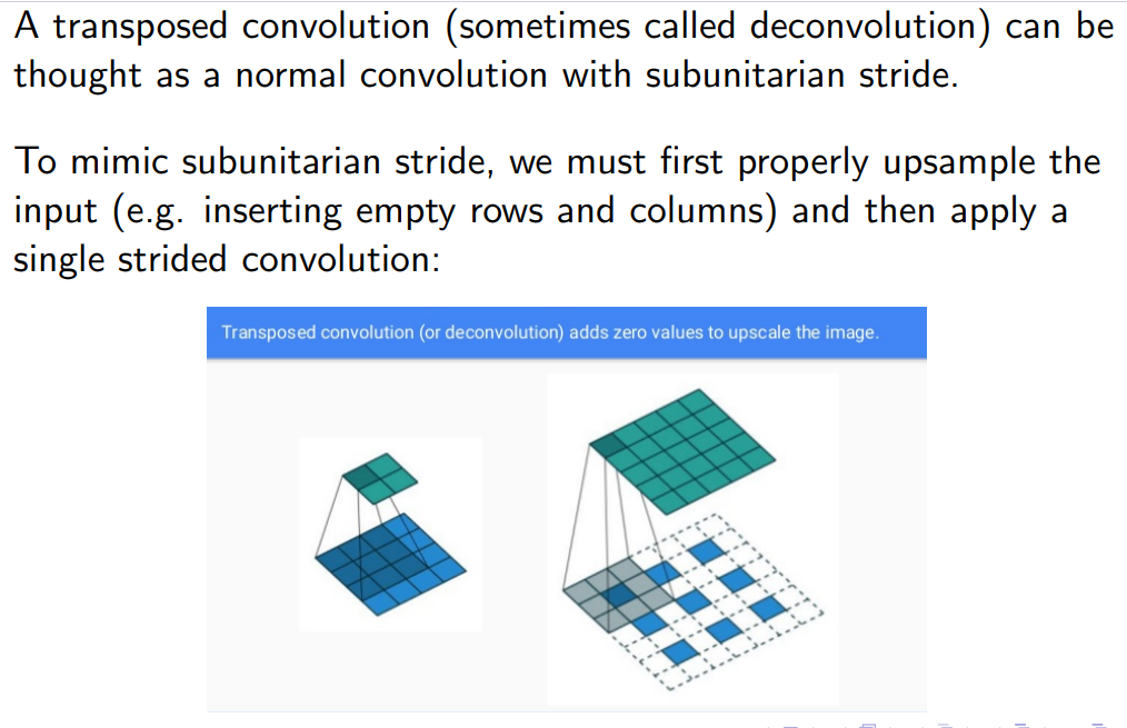
This technique is called transposed convolution because if we transpose the convolution matrix, we see that we are upscaling the input!. Però non ho capito in che modo funziona!

Dilated convolutions

• Slide intuizione di questo

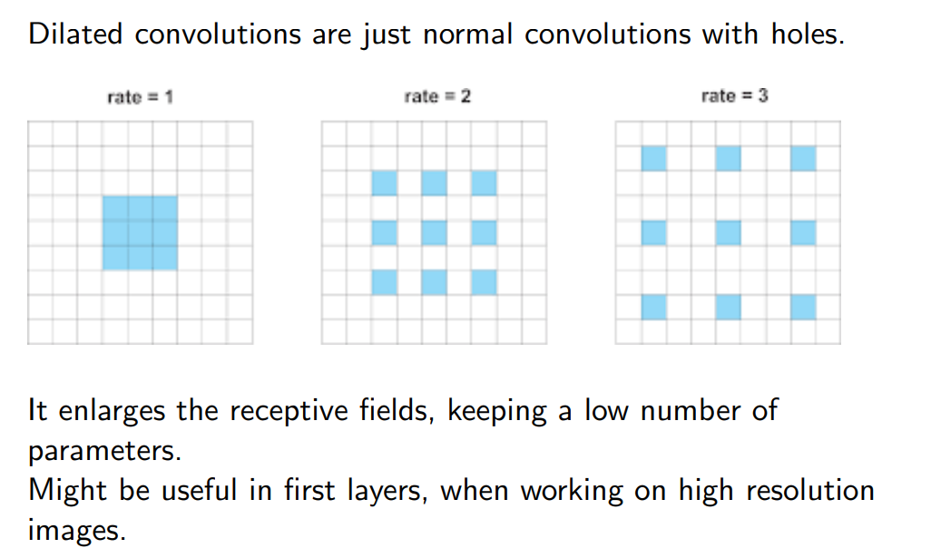
Facciamo una specie di padding interno sul kernel (non vado a contare certe cose, però riesco a ingrandire la receptive field del mio network.

Ha più senso fare sta cosa quando sto analizzando HIGH RESOLUTION IMAGE in cui il valore dei pixel cambia molto poco. Una differenza con le Transposed convolutions (Upconvolution) è il fatto che quelle sono fatte sull’input, questa la facciamo su come viene calcolato il kernel. Sono molto utilizzate in temporal convolution networks, in cui provo a diluire volta per volta lo spazio all’interno del kernel, anche se non so ancora perché va

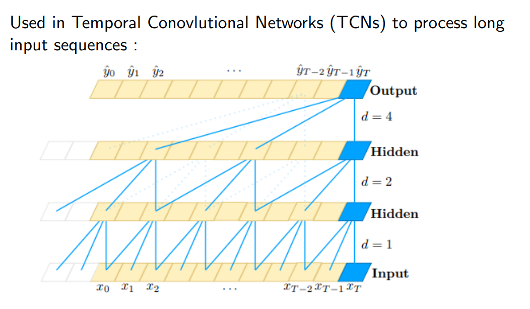This is somewhat similar to what is done in WaveNets, see Autoregressive Modelling

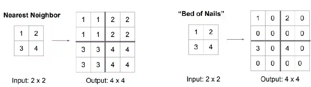
Upsampling

Nearest-neighbor and bed of nails

NN upsampling just repeats the number in the position, while bed of nails is just putting the number in the position and zeroing everything else.

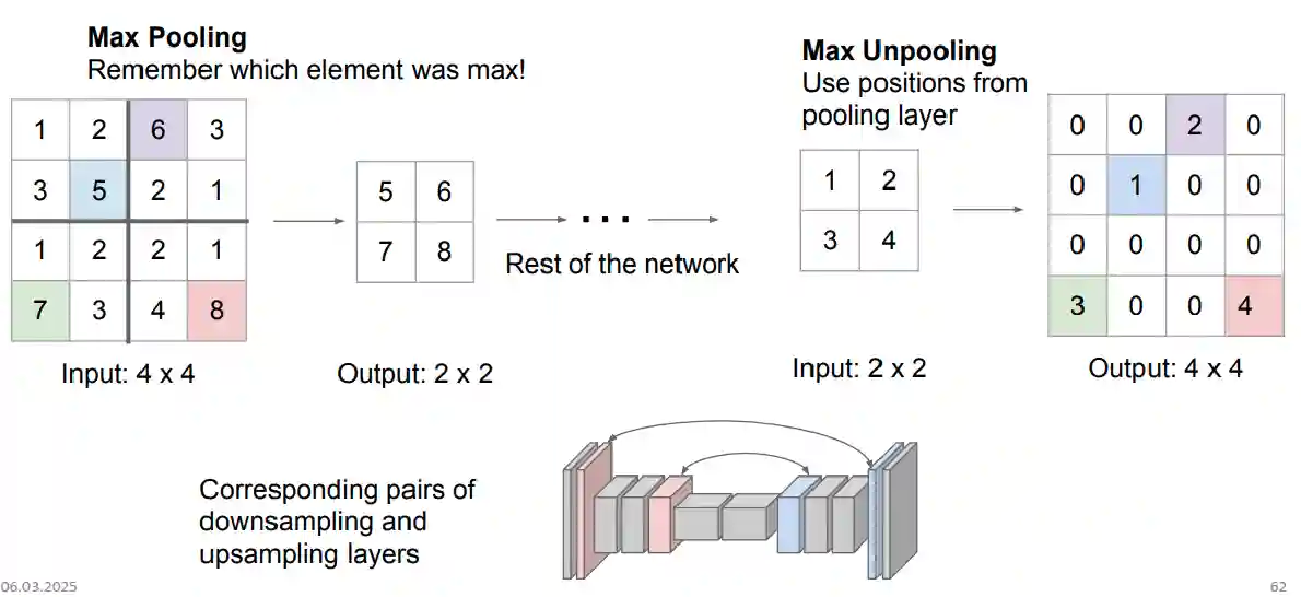
Max-unpooling

You use the equivalent positions of the max-pooling layers, and then put the number in that position there, circled by zeros.

Upconvolution

This is also called transposed convolution. Since normal convolutions can be understood as some matrix $y = Mx$ this is just some other matrix $x = M^{T}y$.

You have the same thing here:

• Strides, kernels, padding
• Sum when the things overlap
• You can also have a learnable kernel (which is an advantage of this method compared to others)

One simple example might explain what upconvolution do: Consider for simplicity a 1D case, with kernel size 3 and stride 2. Suppose input are two numbers $x_{0}$ and $x_{1}$, then the output is $\left[ k_{0}x_{0}, k_{1}x_{0}, k_{2}x_{0} + k_{0}x_{1}, k_{1}x_{1}, k_{2}x_{1} \right]$

Normalization layers

Why normalization

Reasons:

• Have a more stable and faster learning
• More independence between layers (e.g. Layer Norm)

Why is normalization a good idea :D?

• So the quantitative values are comparable from each other (e.g. ages and income)
• We want the output of the layers to be comparable from each other, the middle outputs are inputs for other layers!
• We can better control the activation layers. (non vogliamo che faccia come output NaN 😟)
• Decoupling of the layers. (non dobbiamo andare ad imparare il range di input aspettato, dato che sarà sempre data di stesso tipo)

Batch Normalization

This paper introduces the idea of Batch Normalization.

As each layer observes the inputs produced by the layers below, it would be advantageous to achieve the same whitening of the inputs of each layer. By whitening the inputs to each layer, we would take a step towards achieving the fixed distributions of inputs that would remove the ill effects of the internal covariate shift.

LeCun showed that whitened data speeds up learning, but it was applied only on the input layer. The idea here is to attempt to whiten the input data for every single layer, and this helps. (They call this the internal covariate shift). The thing is that you are learning the normalization parameters.

Probably the internal covariate shift is not the real reason:

Instead BatchNorm fundamentally impacts the training process by making the optimization landscape significantly smoother, thus leading to a more predictive and stable behaviour of the gradients

This is the most common form of normalization (ma l’idea è sempre la stessa, computare varianza e media, e poi sottrarre media e dividere per varianza). La cosa in più è che vengono aggiunte delle varianze e una media, per denormalizzare l’output, in modo che abbia la forma dei dati migliore possibile.

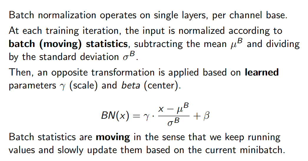
In reality, how it is implemented in pytorch is that $\mu^{B}$ and $\sigma^{B}$ are computed for each batch, and then used to normalize the output, they are not learned parameters. But an weighted average is kept for inference.

Batch normalization makes weights in deeper layers more robust to changes to weights in the shallower layers of the network.

Other Normalization

Potremmo provare a normalizzare per canale

• Slide normalizations

!!

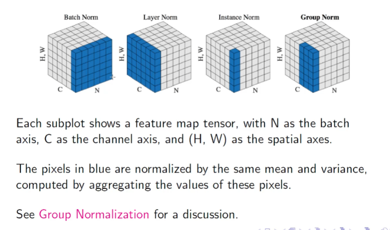
There are many kinds of normalization, here is a table that summarizes the most famous cases.

Name	Normalizes over	Parameters	Dependency on Batch Size	Typical Use Cases
BatchNorm (BN)	(N,H,W)(N, H, W) — per channel	Yes	Yes	Classification, convnets
LayerNorm (LN)	(C,H,W)(C, H, W) — per sample	Yes	No	NLP, transformers
InstanceNorm (IN)	(H,W)(H, W) — per channel per sample	Yes	No	Style transfer, generative models
GroupNorm (GN)	Subsets of channels	Yes	No	General-purpose, batch-size agnostic
PixelNorm	Across channels per pixel	No	No	GANs (especially StyleGAN)

References

[1] He et al. “Deep Residual Learning for Image Recognition” IEEE 2016