Machine learning cannot distinguish between causal and environment features.

Shortcut learning

Often we observe shortcut learning: the model learns some dataset dependent shortcuts (e.g. the machine that was used to take the X-ray) to make inference, but this is very brittle, and is not usually able to generalize.

Shortcut learning happens when there are correlations in the test set between causal and non-causal features. Our object of interest should be the main focus, not the environment around, in most of the cases. For example, a camel in a grass land should still be recognized as a camel, not a cow. One solution could be engineering invariant representations which are independent of the environment. So having a kind of encoder that creates these representations.

Counterfactual Invariance

Counterfactual invariance is a formal framework to define the variables that influence and do not influence the output of a model under certain contexts (i.e. downstream tasks that you could have). It has been introduced in (Veitch et al. 2021) for text perturbations originally.

A first notion of counterfactual invariance

Suppose we have a function $f:\mathcal{X}\to \mathcal{Y}$. Let's define a counterfactual for a random variable $X$. Let's say $W$ is a random variable that represents our non-causal features, e.g. our background. We say $X(\omega )$ is the result of $X$ when $W=\omega$, so we force the background to be some specific thing. We would like to formalize the following idea: the outcome of $X$ should be only dependent on $X$, not on $\omega$.

We say $f$ is counterfactually invariant if the following holds: $f(X(\omega ))=f(X({\omega }^{\prime }))$ for any $\omega ,{\omega }^{\prime }\in W$. How does this happen in practice? Ideally we would like to train any counterfactual, but this is practically impossible (too many resources to get camels into Himalaya to create this counterfactual! Additionally, we have too many possible background environments!)

Causal Graphs

The main advantage of using causal graphs is the intuitive understanding of the relations between the variables. Furthermore, these graph relations could be used to define algorithms for inference that exploit their structure. So we say: causal graphs are both interpretable and useful inference models. We now explore some desiderata that is clearly understood in terms of causal graphs: to correctly formalize the notion of counterfactual invariance.

Causal Graphs

In causal scenarios our input features $X$ indeed have a causal relation with $Y$

Suppose we want to classify cancer and we have three features, $X=(location,C{O}_2,smoke)$, where location is ${\mathbb{R}}^2$, $C{O}_2\in \mathbb{R}$, and $smoke$ is a boolean is our $Y$, or categorical, $W=city$. We can build a causal graph of possible relations between the variables.

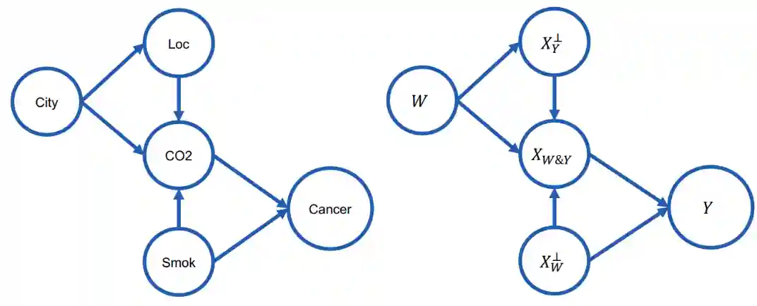
In the above image $X_Y^{\perp }$ is the set of variables that do not influence $Y$, and $X_{W\&Y}$ is the set of variables that influence both $W$ and $Y$. And $X_W^{\perp }$ is the set of variables that are not influenced by $W$ but do influence $Y$.

Anti-Causal

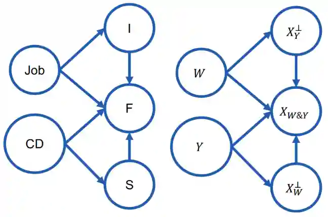
Let's consider another scenario anti-causal scenario, where we want to predict celiac disease, we have stomach ache, fatigue and income as features. Our background variable would be the Job. In these kinds of scenarios, our output random variables $Y$ have a causal relationship with the features in $X$.

Whys of non-causal relations

We can say that two are the main causes of non-causal associations in causal graphs:

1. Confounding variables: existence of another random variable U that could affect both of the variables of our interest.
2. Selection bias: We have a variable S that filters the dataset based on the features that we want.

Where $X$ are the input features , $Y$ are the output, and $W$ is the environment. In this whole set of note we will keep this nomenclature. An example of selection bias is studying the success of jobs, but you just sample from people on LinkedIn. Formally, we say we have a selection bias if all our samples have a selection criteria $S=1$. If we want to account both for confounding variables and selection bias, we say our samples satisfy

$$P(X,Y,Z)=\int P(X,Y,Z,u\mid S=1)du$$

We say that a relationship is purely spurious if

$$Y\perp X\mid W,X_W^{\perp }$$

That is: we can predict $Y$ by only using features that do not depend on $W$. This is a easy way to define spuriousness.

Simpson's Paradox

We give the intuition on this paradox with a simple example. Let's say we have treatment A and B, we would like to know which treatment is better. We sent 350 to A and 350 to B. Let's say we observe that with treatment A $78\%$ recovered, with B $83\%$ recovered. Seems treatment B is better. But in the case we have another variable, e.g. the severity of the illness, the view could be far more different! These are called confounding variables. When designing an experiment we should keep also this in mind.

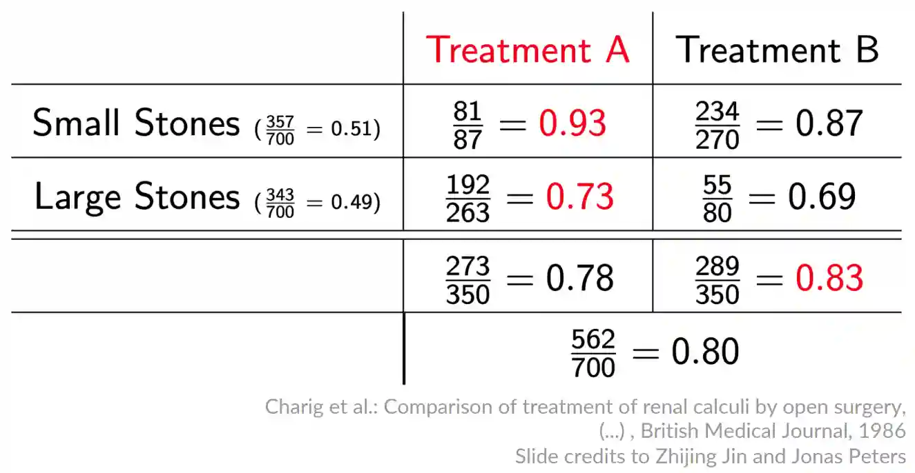
Simpson's paradox occurs due to confounding variables that influence both the group formation and the variables being studied. The decision whether to use treatment $A$ or $B$ should be based on causal considerations for Judea Pearl: different causal structures could arise for the same data, see (Pearl 2009) Chapter 6.1.3.

This phenomenon can be described in terms of events in probability. Consider $E$ to be the variable of effect, $C$ a cause (for example the drug trial) and $F$ an indicator variable describing a sub-population (i.e. Male or Female). We have:

$$\begin{array}{r}P(E\mid C)>P(E\mid C^c)\\ P(E\mid C,F)<P(E\mid C^c,F)\\ P(E\mid C,F^c)<P(E\mid C^c,F^c)\end{array}$$

A formal definition for counterfactual invariance

Intuitively a model $f$ is counterfactually invariant if it only depends on $X_W^{\perp }$ which are the features independent on the background (the cow in the example before). The following has been proven by Veitch in (Veitch et al. 2021), this should be still an active area of research.

For an estimator $f$ to be counterfactually invariant we need:

• Anti-causal scenario $f(X)\perp W\mid Y$
• Causal scenario without selection (possibly confounded) $f(X)\perp W$
• Causal scenario with selection we need $f(X)\perp W\mid Y$ as long as $(X_{W\&Y},X_Y^{\perp })$ do not influence $Y$, i.e. we have $Y\perp X\mid X_W^{\perp },W$ .

Therefore, connecting to the intuitive notion of counterfactual invariance we would like to have $f(X)\mid W=w,Y=y$ to have the same distribution as $f(X)\mid W=w^{\prime },Y=y$ for any $w,w^{\prime }$. It is

V-structures

This is called d-separation.

Let's take for example they are 3 random variables $A,B,C$ in this order. They are all Markov Chains. The nice thing that we have is that

$$p(A,C\mid B)=P(A\mid B)p(C\mid B)$$

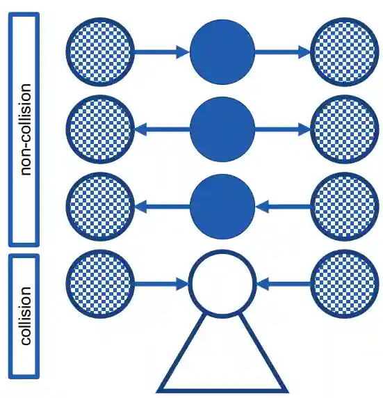
A V structure is a Markov chain in this form $A\to B\leftarrow C$: if i know B, then $A,C$ are related to each other.

For example, suppose we have a chain $A\to B\to C$ which is a Markov chain, and conclude that knowing $B$, makes A and C conditionally independent. Then $p(A,B,C)=P(C\mid B)P(B\mid A)P(A)$, in particular, if we consider $A$ and $C$ we can observe they are conditionally independent given $B$:

$$P(A,C\mid B)=P(C\mid B)\frac{P(B\mid A)P(A)}{P(B)}=P(C\mid B)P(A\mid B)$$

One thing that has not been said about collisions, is that we need every child of it to be not observed (this is what the pyramid below that means).

Similarity Metrics

If we have two $X$ that represent the same idea but in different backgrounds, we would like their two representations to be somewhat similar. This brings the need to create some sort of a metric to measure their similarity. This section attempts to build upon this idea. This seems to be one of the seminal papers on the idea.

Checking the difference

We would like a way to compute a metric that tells us how different two probability distributions are (this is called two sample or homogeneity problem) . Given a probability space $(\mathcal{X},\Sigma ,p^{\ast })$ and another $(\mathcal{X},\Sigma ,q^{\ast })$, and $\mathcal{X}$ is compact. Given some realizations:

$$\begin{array}{r}\{x_1,\dots ,x_n\}\sim p^{\ast }\\ \{y_1^{\prime },\dots ,y_n^{\prime }\}\sim q^{\ast }\end{array}$$

We would like to quantify the sameness between these two distributions. Note that they share the sample space and the Sigma algebra on that.

The idea is that if $p\ne q$ then there exists a set in the sigma algebra that has different measure (else, it would be exactly the same). We can write the same thing with the use of expectation as:

$$p^{\ast }(x)\ne q^{\ast }(x)⟹{\mathbb{E}}_{p^{\ast }}[1_A(x)]]\ne {\mathbb{E}}_{q^{\ast }}[1_A(x)]]$$

The indicator can be approximated by a continuous trapezoidal function with very high slope.

$$\exists f\in C(x):{\mathbb{E}}_{p^{\ast }}[f(x)]\ne {\mathbb{E}}_{q^{\ast }}[f(x)]$$

So checking the difference is the same as computing the expectation of the approximation of the indicator function. This has been formally proven by Dudley (2002) lemma 9.3.2 (they have proved something stronger).

Comparison with KL Divergence

This section was generated by GPT.

Feature	MMD	KL Divergence
Requires explicit densities	No	Yes
Symmetry	Symmetric	Asymmetric
Support mismatch	Well-defined	Can be infinite
Computational feasibility	Efficient for empirical samples	Challenging for high-dimensional data
Robustness to noise	Robust	Sensitive

MMD is ideal in situations where:

1. You only have empirical samples of the distributions.
2. The distributions are high-dimensional and nonparametric.
3. A symmetric or support-insensitive measure is needed.

Maximum Mean Discrepancy

The Maximum Mean Discrepancy is a way to measure the difference between two distributions that builds upon the previous idea. It is defined as:

$$MMD(\mathcal{F},\mathcal{X},\mathcal{Y})=\underset{f\in \mathcal{F}}{\sup }\left|{\mathbb{E}}_{x\sim p}[f(x)]-{\mathbb{E}}_{y\sim q}[f(y)]\right|$$

Where $\mathcal{F}$ is a set of functions that are bounded and continuous. The MMD is a metric that measures the difference between two distributions (Müller 1997). The bad thing is that it is difficult to compute: the space of the functions is quite large. In this discussion we will restrict ourselves to the unit sphere of universal RKHS, see Kernel Methods for that. One interpretation of this set is the polynomials whose coefficients squared is 1.

Riesz Representation Space

Applying a bounded linear operator in a Hilbert's Space, then the operator can be represented as a inner product with a function in the space. This is the Riesz Representation Theorem in short! The main usage is moving from the functional realm to an algebraic realm. So we have a strong connection between functional analysis and algebra!

Formally, it states that for every linear functional $L$ on $H$, a Hilbert's Space, there exists a unique vector $v$ in $H$ such that

$$L(u)=⟨u,v⟩$$

And the norm of the functional is the norm of the vector. In this context, we use it to say that we can write

$${\mathbb{E}}_{\mathcal{X}}[f(x)]={\beta }_f^T{\mu }_{\mathcal{X}}$$

Algebraic Maximum Mean Discrepancy

We will use Riesz representation theorem and the above MMD to come up with an algebraic version of it that should be easier to compute. By Riesz theorem, computing $f(x)$ is the same as computing the inner product with $\varphi (x)\in RKHS$ where $\varphi$ is from a family of functions in the RKHS (See Kernel Methods). We express this version of MMD in the following way (Lemma by Borgwardt et al. 2006):

$$\begin{array}{rl}MM{D}^2(\mathcal{F},\mathcal{X},\mathcal{Y})& ={\left[\underset{\Vert f{\Vert }_{\mathcal{H}}\le 1}{\sup }({\mathbb{E}}_p[f(x)]-{\mathbb{E}}_q[f(y)]\right]}^2\\ \text{Using Riesz Th. }& ={\left[\underset{\Vert f{\Vert }_{\mathcal{H}}\le 1}{\sup }({\mathbb{E}}_p[⟨\varphi (x),f{⟩}_{\mathcal{H}}]-{\mathbb{E}}_q[⟨\varphi (y),f{⟩}_{\mathcal{H}}]\right]}^2\\ \text{Using linearity of expectation}& ={\left[\underset{\Vert f{\Vert }_{\mathcal{H}}\le 1}{\sup }⟨{\mu }_{\mathcal{X}}-{\mu }_{\mathcal{Y}},f{⟩}_{\mathcal{H}}\right]}^2=\underset{\Vert f{\Vert }_{\mathcal{H}}\le 1}{\sup }{\left[⟨{\mu }_{\mathcal{X}}-{\mu }_{\mathcal{Y}},f{⟩}_{\mathcal{H}}\right]}^2\\ \text{Using Chauchy Schwarz}& =\underset{\Vert f{\Vert }_{\mathcal{H}}\le 1}{\sup }\Vert {\mu }_{\mathcal{X}}-{\mu }_{\mathcal{Y}}{\Vert }_{\mathcal{H}}^2\Vert f{\Vert }_{\mathcal{H}}^2=\Vert {\mu }_{\mathcal{X}}-{\mu }_{\mathcal{Y}}{\Vert }_{\mathcal{H}}^2\\ & =⟨{\mu }_p,{\mu }_p{⟩}_{\mathcal{H}}+⟨{\mu }_q,{\mu }_q{⟩}_{\mathcal{H}}-2⟨{\mu }_p,{\mu }_q{⟩}_{\mathcal{H}}\\ & ={\mathbb{E}}_p[k(x,x^{\prime })]+{\mathbb{E}}_q[k(y,y^{\prime })]-2{\mathbb{E}}_{p,q}[k(x,y)]\end{array}$$

The nice thing is that the latter form can be empirically approximated:

$${\mathbb{E}}_{x,x^{\prime }\sim p}[k(x,x^{\prime })]\approx \frac{1}{n^2}\sum _{i,j}k(x_i,x_j)$$

And the last two are also compute accordingly.

References

[1] Veitch et al. “Counterfactual Invariance to Spurious Correlations in Text Classification” Curran Associates, Inc. 2021

[2] Pearl “Causality” Cambridge University Press 2009