The Potassium Exchange values
We use the measurement by Cole and Curthis 40mS/cm squared was their measure of Potassium ions leaving the membrane
$$ \Delta Q = Idt = GA \Delta E dt $$The potassium concentration is 0.155 moles per litre. Where $G$ is the conductance per unit area, $A$ the membrane surface, $E$ voltage deflection Remember that the conductance is the reciprocal of the resistance, and $V = IR \implies I = \frac{V}{R} = GV$
Assuming for the radius $r$ of our cylindrical axon $r = 1\mu$m $(A = 2\pi r l, V = \pi r^2 l)$, the potassium concentration $[\text{K}^+]_i = 0.155 \text{ M/l}$, the action potential duration $dt = 1 \text{ ms}$, the action potential amplitude $\Delta E = 0.1 \text{ V}$, we get using Faraday’s constant $F \simeq 10^5 \text{ C/M}$ that:
$$ \frac{\Delta Q}{Q} = \frac{2G \Delta E dt}{[\text{K}^+]_i F r} \simeq 0.5\%. $$So we discover that the main part of potassium stays inside.
Typical membrane potentials
$$ V_{T} = \frac{RT}{F} $$Where $R$ is the gas constant, $T$ the temperature, $F$ Faraday’s constant. Is the thermal voltage formula. at body temperature we have: $$ \begin{align*} V_T &= \frac{(8.314 \ \text{J/(mol·K)}) \cdot (310 \ \text{K})}{96,485 \ \text{C/mol}}\ V_T &= \frac{2,577.34 \text{ V·C}}{96,485 \text{ C}} = 0.0267 \text{ V} = 26.7 \text{ mV} \end{align*}
$$ $$V_T = \frac{(8.314)(310)}{96,485} \approx 26.7 \text{ mV} $$
Typical living creatures range -3 to 2 values. In humans it is 70mV
Leaky Integrate and fire neuron
Presynaptic fire -> post synaptic fire means strenghtening of connection. Opposite is making connection weaker. Esponentially decaying memory of firing of the neuron (this is some sort of a trace). And reading out at different moment gives the two things.
Spike Timing Dependent Plasticity
• Synaptic Modification: STDP is a mechanism for modifying synaptic strength, which can lead to either Long-Term Potentiation (LTP) or Long-Term Depression (LTD). • Timing Dependence: The direction and magnitude of synaptic change are typically dependent on whether the presynaptic spike occurs just before or just after the postsynaptic spike We have seen something familiar in the potentiation of the Schaffer Collateral in Memory in Human Brain.
Backpropagation in SNN: da finire.
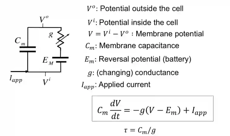
Reminder of RC circuits
Remember that the equation for RC circuits is:
$$ \tau \frac{dV(t)}{dt} = -V(t) + V_{\text{rest}} + RI(t) $$Resistance and capacitor tell us how much time will be needed before I have full charge. This is easily derivable from the equation of current in time.
$$ V = IR $$$$ Q= CV $$They have a rate code of time-difference. This is how neurons do encode this part. Rate Code or temporale code are the two main theories.
Rate code vs Temporal Code
Rate-code: The information a neuron transmits is encoded in the average firing rate, which means how many spikes it produces in a given time window. Temporal-code: The precise timing of spikes, down to millisecond precision, carries information, not just the firing rate. The specific activity pattern in time carries information.
Cortical areas are usually outer encoded, meaning a population of neurons encode features, while higher and deeper level neurons are usually linear, and encode simple features. One example are place neurons studied in Memory in Human Brain
Equivalent circuit model of a membrane patch
$$ I(t) = \frac{u(t) - u_{\text{rest}}}{R} + C \frac{du(t)}{dt} $$$$ u(t) = u_{\text{rest}} + \Delta u \exp\left( - \frac{t - t_{0}}{\tau_{m}} \right) $$If the entire surface of an axon were insulated, there would be no place for current to flow out of the axon and action potentials could not be generated.
Which is called the free solution, useful to model passive membrane models.
$$ v = \frac{V - V_{L}}{V_{\theta} - V_{0}}, i_{app} = \frac{I_{app}}{g_{L}(V_{\theta} - V_{0})} $$$$ \tau \frac{dv}{dt} = -v + i_{app} $$$$ f = \frac{1}{\tau} \left[ \log \left( 1 + \frac{1}{i_{app} - v_{\theta}} \right) \right] ^{-1} $$When $i_{app} > v_{\theta}$.
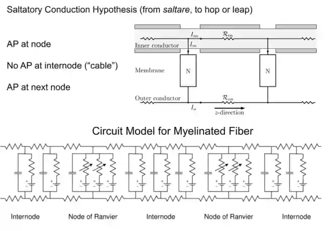
Saltatory Condution Hypothesis
This model is useful to model myelinated membranes.
The Cable Equation
I’ll solve the cable equation step by step to derive the solution V(x) shown in the slide.
Let’s start with the fundamental equations from the circuit model:
- From voltage drop: $$\Delta V = -j_ir_i\Delta x \implies \frac{\partial V}{\partial x} = -j_ir_i$$
- From current: $$\Delta j_i = -j_m\Delta x$$
- And membrane current: $$j_m = V/r_m$$
- Combining these equations: First, take derivative of the voltage equation with respect to x: $$\frac{\partial}{\partial x}(\frac{\partial V}{\partial x}) = -\frac{\partial j_i}{\partial x}r_i$$
- $$\frac{\partial j_i}{\partial x} = -j_m = -\frac{V}{r_m}$$
- $$\frac{\partial^2 V}{\partial x^2} = \frac{r_i}{r_m}V$$
- $$\frac{\partial^2 V}{\partial x^2} - \frac{r_i}{r_m}V = 0$$
-
This is a second-order linear differential equation. Let’s solve it:
- The characteristic equation is: $$m^2 - \frac{r_i}{r_m} = 0$$
- Define $$\lambda = \sqrt{\frac{r_m}{r_i}}$$ (this is the electrotonic length)
- Then general solution is: $$V(x) = Ae^{x/\lambda} + Be^{-x/\lambda}$$
- $$V(x) = Be^{-x/\lambda}$$
- $$V(x) = e^{-x/\lambda}$$
is the electrotonic length.
This solution shows how voltage decays exponentially along the passive membrane, with λ determining the characteristic length scale of the decay.
Both resistivities are dependend on the area. (inverse of that).
Integrating Synapses
$$ C \frac{dV_i}{dt} = -g_{L_i} (V_i - V_L) - \sum_j g_{ij} (V_i - V_{ij}) + I_{\text{app}} $$It’s easier to see each contribution as $I_{j}$
where:
- $V_{ij}$: reversal potential of synapses
- $V_{ij} > V_{\theta}$: excitatory,
$V_{ij} < V_{\theta}$: inhibitory - $g_{ij}$: synaptic conductance
- ’tug of war between batteries'
Which is a simple extension of the integrate and fire model with more currents defined by the $g$ value.
Leaky integrator model
The Leaky is the threshold reset equation with the equivalent circuit model for the neuron. The main idea of this model is the reset of the membrane potential after firing, the RC membrane circuit model and similar things.
Threshold resetting means putting the $V$ value back at a certain $V$ value when it is above a certain threshold.
$$ f \approx \frac{[I_{app} - gL(V_{1/2} - V_L)]^+}{C(V_\theta - V_0)} $$Where we have a numerator in the Relu.
Rate based approximator
The firing rate is not the slowly responding variable, it is instantaneous. The synaptic activation slowly reacts to the firing rate. This is the rate-based approximation of the membrane conductance.
$$g_{syn} \leftarrow g_{syn} + \frac{\alpha}{\tau}$$$$\tau \frac{dg_{syn}}{dt} + g_{syn} = 0$$$$\tau \frac{dg_{syn}}{dt} + g_{syn} = \alpha\sum_j \delta(t-t_j)$$$$\simeq \alpha F$$Where F represents the firing rate, as indicated in the image. The method uses averaging over the fast variable.
Firing rate of a Neuron
After it fired the first time, making it fire again requires a charge difference of $C(V_{\theta} - V_{0})$. We need to solve the capacitor recharge equation to get that value:
$$ \begin{align*} T &\;=\; \int_{V_0}^{V_\theta} \frac{C\,dV}{I_{\text{app}} \;-\; g_L\,[\,V - V_L\,]}\\ &=\; \int_{V_0}^{V_\theta} \frac{C\,dV}{I_{\text{net}} \;-\; g_L\,V} \;=\; \frac{C}{g_L}\;\ln \!\biggl[\, \frac{I_{\text{net}} \;-\; g_L\,V_0}{\,I_{\text{net}} \;-\; g_L\,V_\theta} \biggr].\\ &\implies f \;=\; \frac{1}{T} \;=\; \biggl[\;\frac{C}{g_L}\;\ln \!\Bigl(\! \frac{I_{\text{net}} \;-\; g_L\,V_0}{\,I_{\text{net}} \;-\; g_L\,V_\theta} \Bigr)\biggr]^{-1}. \\ & = \biggl[\;\frac{C}{g_L}\;\ln \!\Bigl(\! 1 +\frac{g_L(V_{\theta} - V_0)}{\,I_{\text{net}} \;-\; g_L\,V_\theta} \Bigr)\biggr]^{-1} \end{align*} $$Which is our firing rate.
$$ f\;\approx\; \frac{1}{T} \;=\; \frac{\bigl[I_{\text{app}} - g_L\,\bigl(V_{1/2} - V_L\bigr)\bigr]^+} {C\,\bigl(V_\theta - V_0\bigr)}, $$Probabilistical Models for Synapses
At neuromuscular junctions, acetylcholine is released randomly into the cleft even without any synapse. The motor end plate receives these signals and is passively stimulated.
End Plate Potentials
Synapses change slightly the potentials in the post synaptic neuron. Sometimes there are mini potentials that are not enough to trigger an action potential.
These potential amplitudes could be modeled by a binomial distribution. All the MEPP are unimodal about 0.4mV. While the EPP are multimodal.
$$ P_{k} = \binom{n}{k} p^{k} (1-p)^{n-k} $$And this gives a good fit of it.
Miniature End Plate Potentials
Miniature end-plate potentials (MEPPs) are the tiny depolarizations recorded at the muscle end plate in the absence of nerve stimulation, of about 1mV (while normal EPP are of 40-50 mV).
They are the “background noise” of neurotransmission, but in fact they reveal something very fundamental: that acetylcholine (ACh) is released in discrete packets (quanta), even without action potentials.
Summed together, many vesicles released simultaneously during a real presynaptic action potential → a full EPP → muscle contraction.
This was an important experiment to prove the quantization of the vesicles in 1950
Quantas and Vesicles fusing
We have that there is a linear correlation between fusing of vesicles and quantas that are released. The number of quanta released has beenestimated by fitting a binomial model to intracellular recordings.