A simple motivation
Fisher’s Linear Discriminant is a simple idea used to linearly classify our data.

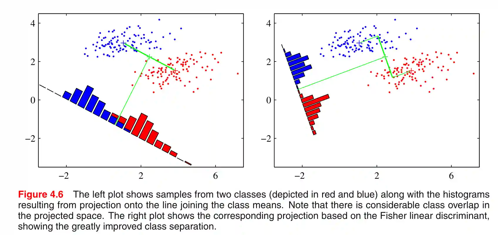
The image above, taken from (Bishop 2006), is the summary of the idea. We clearly see that if we first project using the direction of maximum variance (See Principal Component Analysis) then the data is not linearly separable, but if we take other notions into consideration, then the idea becomes much more cleaner.
A first approach
$$ m_{j} = \frac{1}{N_{j}}\sum_{i : y_{i} = j} x_{i} $$$$ \arg\max_{w} w^{T}(m_{2} - m_{1}) + \lambda (\lVert w \rVert _{2}^{2} - 1) $$Then we find a solution $w \propto (m_{2} - m_{1})$.
But the problem with this formulation is that we could have some strong overlap in the projected domain, due to non diagonal covariances in the class distribution. We would also like to minimize the within class variance during the projection, so that we can better separate the two values.
Adding inter-class variance
$$ s_{i}^{2} = \sum_{n \in \mathcal{C}_{i}} (w^{T}x_{n} - w^{T}m_{n})^{2} $$We simply compute the inter-class variance and divide, getting the Fisher discriminant
$$ J(w) = \frac{w^{T}(m_{2} - m_{1})^{2}w}{s_{1}^{2} + s_{2}^{2}} = \frac{w^{T}S_{B}w}{w^{T}S_{I}w} $$The lower part is the sum of the within class variances, while the upper part is the between class covariance.
Now, if we do some calculus we find that the best solution is $w \propto S^{-1}_{w}(m_{2} - m_{1})$
Code example
Code example nicely produced by Claude. Checked by Human.
import numpy as np
import matplotlib.pyplot as plt

class FisherLDA:
    def __init__(self, n_components=1):
        """
        Initialize Fisher's Linear Discriminant Analysis

        Parameters:
        n_components (int): Number of components to keep (usually 1 for binary classification)
        """
        self.n_components = n_components
        self.w = None  # Projection vector

    def fit(self, X, y):
        """
        Fit the LDA model according to Fisher's criterion

        Parameters:
        X: array-like of shape (n_samples, n_features)
        y: array-like of shape (n_samples,) - Class labels
        """
        # Split data by class
        X0 = X[y == 0]
        X1 = X[y == 1]

        # Calculate class means
        mean0 = np.mean(X0, axis=0)
        mean1 = np.mean(X1, axis=0)

        # Calculate within-class scatter matrix Sw
        S0 = np.zeros((X.shape[1], X.shape[1]))
        S1 = np.zeros((X.shape[1], X.shape[1]))

        for x in X0:
            x = x.reshape(-1, 1)
            S0 += (x - mean0.reshape(-1, 1)) @ (x - mean0.reshape(-1, 1)).T

        for x in X1:
            x = x.reshape(-1, 1)
            S1 += (x - mean1.reshape(-1, 1)) @ (x - mean1.reshape(-1, 1)).T

        Sw = S0 + S1

        # Calculate between-class scatter matrix Sb
        mean_diff = (mean1 - mean0).reshape(-1, 1)
        Sb = mean_diff @ mean_diff.T

        # Calculate optimal projection vector w
        # w ∝ Sw^(-1)(μ1 - μ0)
        try:
            self.w = np.linalg.inv(Sw) @ (mean1 - mean0)
            # Normalize the projection vector
            self.w = self.w / np.linalg.norm(self.w)
        except np.linalg.LinAlgError:
            # If Sw is singular, use pseudoinverse
            self.w = np.linalg.pinv(Sw) @ (mean1 - mean0)
            self.w = self.w / np.linalg.norm(self.w)

        return self

    def transform(self, X):
        """
        Project the data onto the most discriminative direction

        Parameters:
        X: array-like of shape (n_samples, n_features)

        Returns:
        X_transformed: array-like of shape (n_samples, n_components)
        """
        return X @ self.w

# Demonstration
if __name__ == "__main__":
    # Generate sample data
    np.random.seed(42)
    n_samples = 100

    # Class 0
    mean0 = [0, 0]
    cov0 = [[1, 0.5], [0.5, 1]]
    X0 = np.random.multivariate_normal(mean0, cov0, n_samples)

    # Class 1
    mean1 = [2, 2]
    cov1 = [[1, 0.5], [0.5, 1]]
    X1 = np.random.multivariate_normal(mean1, cov1, n_samples)

    # Combine data
    X = np.vstack([X0, X1])
    y = np.hstack([np.zeros(n_samples), np.ones(n_samples)])

    # Fit LDA
    lda = FisherLDA()
    lda.fit(X, y)

    # Transform data
    X_transformed = lda.transform(X)

    # Plotting
    plt.figure(figsize=(12, 5))

    # Original data
    plt.subplot(121)
    plt.scatter(X0[:, 0], X0[:, 1], label='Class 0')
    plt.scatter(X1[:, 0], X1[:, 1], label='Class 1')
    plt.arrow(0, 0, lda.w[0], lda.w[1], color='r', width=0.05, label='Projection direction')
    plt.xlabel('Feature 1')
    plt.ylabel('Feature 2')
    plt.title('Original 2D Data with LDA Direction')
    plt.legend()

    # Projected data
    plt.subplot(122)
    plt.hist(X_transformed[y == 0], bins=20, alpha=0.5, label='Class 0')
    plt.hist(X_transformed[y == 1], bins=20, alpha=0.5, label='Class 1')
    plt.xlabel('Projected Values')
    plt.ylabel('Frequency')
    plt.title('Projected Data on Fisher Direction')
    plt.legend()

    plt.tight_layout()
    plt.show()
References
[1] Bishop “Pattern Recognition and Machine Learning” Springer 2006