This is also known as Lagrange Optimization or undetermined multipliers. Some of these notes are based on Appendix E of (Bishop 2006), others were found when studying bits of rational mechanics. Also (Boyd & Vandenberghe 2004) chapter 5 should be a good resource on this topic.
Let's consider a standard linear optimization problem
\begin{array} \\ \min f_{0}(x) \\ \text{subject to } f_{i}(x) \leq 0 \\ h_{j}(x) = 0 \end{array}Lagrangian function
And let's consider the Lagrangian function associated to this problem defined as
We want to say something about this function, because it is able to simplify the optimization problem a lot, but first we want to study this mathematically.
We call the lagrange multipliers associated with their function, where we have that and are free. We can also define the dual function as .
Motivation
In this section we try to explain step by step why this method works. We will find that it is easier than we could expect this. With this, we will evaluate the maximum (for the minimum just take the dual)
Single Equation constraint
In this case we have our function along with a constraint where is a constant in and is a vector. Note: we use but it's the same if just define and you have your other function compared to a 0, which is usually easier in this context. Let's consider the solutions of , this usually gives us a set of points (sometimes contiguous) where we have to look for a solution of , we want to find among these points the one that minimizes the function . The constraint on is somewhat similar to convex analysis' level sets. One thing that is easily observable (this way is very physicist's way to motivate things, you do something similar when analyzing the parallel electric field in conductors see Condensatori nel vuoto), is that if you have a and you move slightly along the path of the value is the same, so the derivative along this direction is null. This allows us to say that the derivative of is perpendicular to the direction of the curve. Formally, we can write the Taylor expansion of around some point :
Then we say that because they both lie in the same contour surface which implies in that direction. So, only the perpendicular component of the gradient remains.
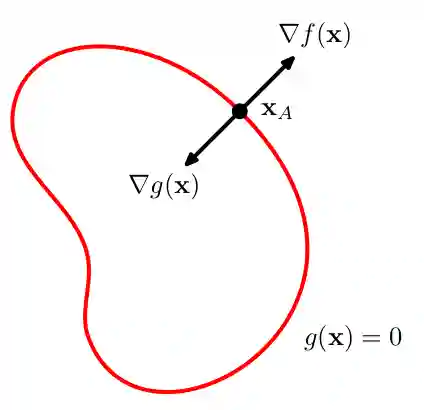 Then we can also say something about the gradient of , because if it is not perfectly perpendicular to that surface, we would have that moving slightly along the surface could increase or decrease the value of . So we need the two to be parallel or anti-parallel. Which motivates us to write which in turn motivates the creation of the so called lagrangian function:
We observe that its stationary point needs to have its partial derivatives set to zero, so we would have the original partial derivative condition, and also the inequality constraint for . In this way we can find both the and the .
In the case we want to minimize, we can choose the lagrangian to be
So that the derivative has opposite direction. (actually I don't have understood this point).
Another intuition
The parameters for the Lagrange Optimization objective can be easily inferred if you remember this short story:
Suppose you are a human and can just live in a rounded disk. Outside is fire, so you cannot go outside. You cannot fly, so you are obliged to stay on the disk ( equality constraint). You cannot leave your disk, so you need to stay within some other inequality constraint. You would like to minimize the distance to a flying thing UFO. If you now consider three scenarios, namely:
- UFO on your disk
- UFO inside the area of your disk but flying at some altitude.
- UFO outside your disk.
Then you see that in the first case, we can satisfy the disk constraints, and just go directly to the UFO, which is classical optimization problem, just set the derivative to 0. In the second case, you need to find the best location in the disk. So it will be directly below or on the UFO. You will see that the two gradients of and align or are anti-aligned. This is the above condition. In the third case, as it is outside, you would like to get as close to the boundary as possible, and the third gradient's parameter should be positive, as it is pointing outside, while the others could be mis-aligned.
Inequality constraints
If instead of having bounds like we have bounds like it's just a little bit more complicated, we have more points, and could be useful to divide the case when with . In the latter case, we just set (because this is what we get if we take the derivative w.r.t. to and set ) and maximize the lagrangian (doesn't matter the direction of the gradient of now), when the solution is border, we should take a little bit more care: we want the gradient of to be away from the region , which motivates us to have an equation like and .
Karush-Kuhn-Tucker Conditions
So we have the same Lagrangian as before, but we have some other constraints, those are called the Karush-Kuhn-Tucker conditions:
The last condition is called complementary slackness conditions.
We can work the four cases intuitively and get some other intuition about Lagrange optimizations. In the (Bishop 2006) there is quite good argumentation that naturlly exposes this part.
Playbook for Lagrange Multipliers
Given an optimization problem
\begin{array} \\ \mathop{\min}_{w} &f(w) \\ \text{ s.t. } &g_{i}(w) \leq 0 \\ &h_{i}(w) = 0 \end{array}- Write the Lagrangian function
with these are the classical conditions, motivated above (just note the minimization problem, so we inverted one condition). 2. Check for Slater's condition which is check if there is a such that for every
- Solve , and
Duality
Primal problem
The Lagrangian Multiplier method allows us to define the concept of dual optimization problem also in this context. If we consider this classical optimization problem
\begin{array} \\ \min_{w} f(w) \\ \text{ s.t. } g_{i}(w) \leq 0 \\ h_{i}(w) = 0 \end{array}We can build the Lagrange Multiplier as
with , these are the classical conditions, motivated above. Now consider this primal value:
We observe that if any of the condition or is violated, then it's easy to say that .
So we say that this formulation is the same as the above:
The dual of this optimization problem is just inverting the values in some manner. We easily notice the following:
This is the trick that makes the Lagrangian work! If we find a closed solution that optimizes the Lagrangian, we can be sure that that is a valid solution for the original problem.
Weak duality
Consider the Lagrangian given the optimization problem above
Given a candidate of the optimization problem, we say that, after fixing and then it's always true that
This is called weak duality: we observe that each possible solution is bounded below by the dual function. When Equality holds for the best and we say that we have strong duality, which implies that the admissible that we have found is actually the best solution possible, and that solving the dual problem actually gives you the best solution for the primal problem.
Dual problem
Dual problem of the Lagrange function is the following:
We can prove some properties of this new function. Note that the chosen could also be a not admissible solution in this case. For weak duality, we know that this is a lower bound for the solution of the primal problem.
So now the optimization problem is
We see a nice symmetry with the primal optimization problem. This is the same as solving
Slater's condition
Slater's condition enables us to assert that strong duality is possible, and thus we have a manner to find the best solution for the optimization problem by optimizing the dual problem. if given the following optimization problem
\begin{array} \\ \min f(w), & w \in \mathbb{R}^{d} \\ \text{ s.t. } g_{i}(w) = 0, & i \leq m \\ h_{j}(w) \leq 0 & j \leq n \end{array}And we have that are all convex and is affine, then this theorem asserts that
if there is a feasible such that for all then we have strong duality.
When we have strong duality, we can solve the dual problem instead of the original problem, as the solution for one, is solution for the other. Recall that strong duality asserts that there is no gap between the primal and the dual problem, and that the solution for one is the solution for the other.
References
[1] Bishop “Pattern Recognition and Machine Learning” Springer 2006
[2] Boyd & Vandenberghe “Convex Optimization – Boyd and Vandenberghe” 2004