In general we want to understand how neurons encode the rate and temporal information to build specific features like place cells, grid cells, velocity, head direction, or how it can guide behaviour or coordination. Many neurons encode together some features, it is quite rare that you have the face neuron and similars. Imaging techniques help us to get more information about these parts.
Basics of Microscopy

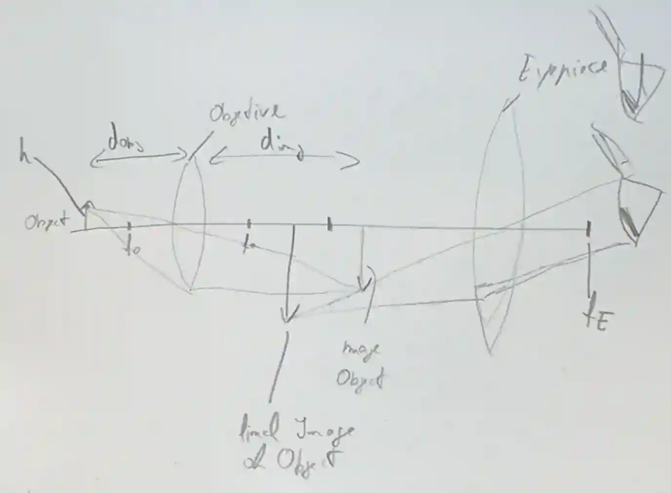
Image of a classical microscope, from course slides
The optical Principle
The basic idea is to have one first lens that makes an object bigger but inverted, and another lens, called the eyepiece that sees the original part bigger, and in correct shape. With some high school physics is possible to compute how much is the enlargement due to the lens.
Lens Physics
$$ \frac{1}{f} = \frac{1}{d_o} + \frac{1}{d_i} $$$$ M = \frac{d_i}{d_o} $$Where $d_{o}$ is the distance of the object to the first lens, and $d_{i}$ is the distance of the image to the first lens.
The two magnifications compound with each other, giving a final value of $M = m_{1} + m_{2}$.
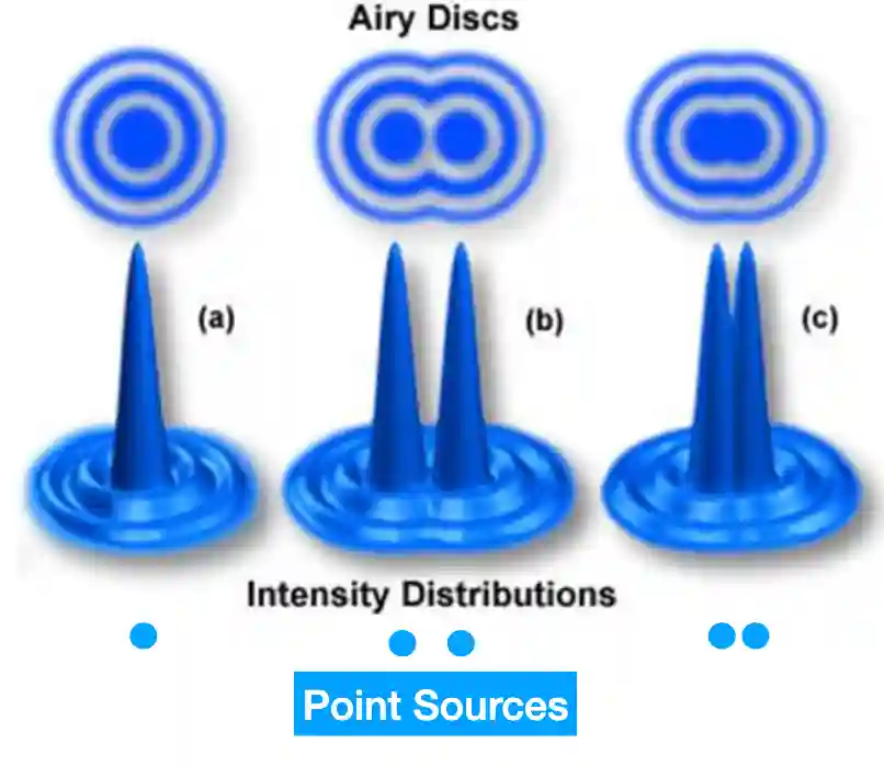
 #### Rayleigh Criterion
This criterion, closely related to image resolution, is defined as:
> The limit at which two Airy disks can be resolved into separate entities.
#### Rayleigh Criterion
This criterion, closely related to image resolution, is defined as:
> The limit at which two Airy disks can be resolved into separate entities.
 $$
\Delta x = \frac{1.22 \cdot \lambda}{2NA}
$$$$
NA = n \cdot sin(\theta)
$$
$$
\Delta x = \frac{1.22 \cdot \lambda}{2NA}
$$$$
NA = n \cdot sin(\theta)
$$Where $n$ is the index of refraction of the medium, and $\theta$ is the angle of the light cone that enters the lens.
Two main things in this formula:
- Wavelength
- Amplitude of the light (low NA means lower resolution).
This means we cannot distinguish two objects that are closer than $\Delta x$, and this is the limit of the resolution of the lens.
Looking at the aperture you can observe that if you are closer (wider aperture angle), then you resolution is higher, but less field of view. Sometimes is not very easy to bring the object to the tissue (bone, some 3d structure e.g.).
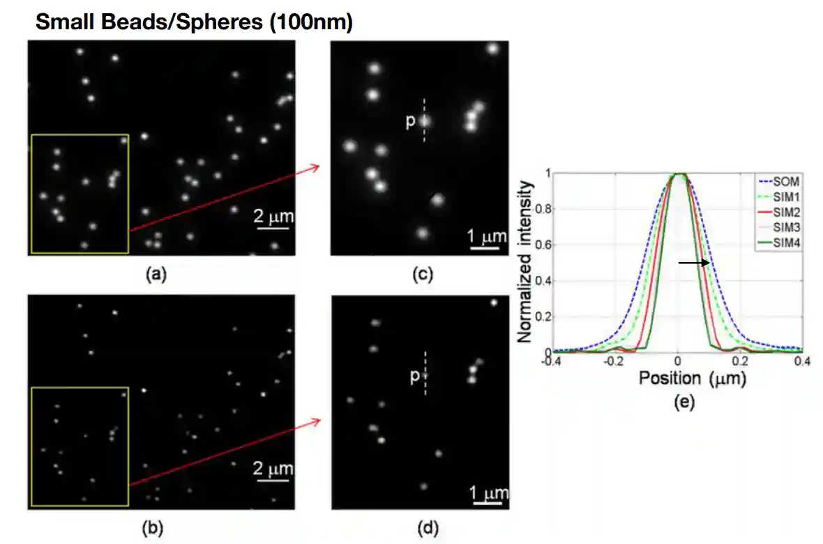
Measuring resolution
In the lab the resolution of a microscope is measured using small beads and spheres of 100nm, we define the resolution as the width of the blurred dots that are produced by the lens.
Types of microscopy
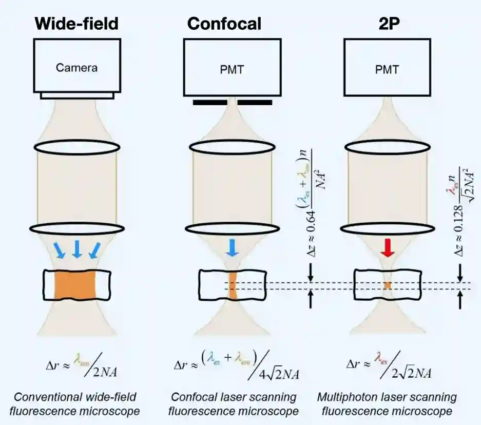
Different microscopes
Electron Microscopy
We have a wavelength of nanometers (meaning we have a nice resolution), which means the resolution is orders of magnitude better than the light microscopy.
We use magnets as lenses in this case.
Nice thing about scanning electron microscopy is that you can gather 3D information (scattering can be seen at different angles), and the resolution is much better than light microscopy.
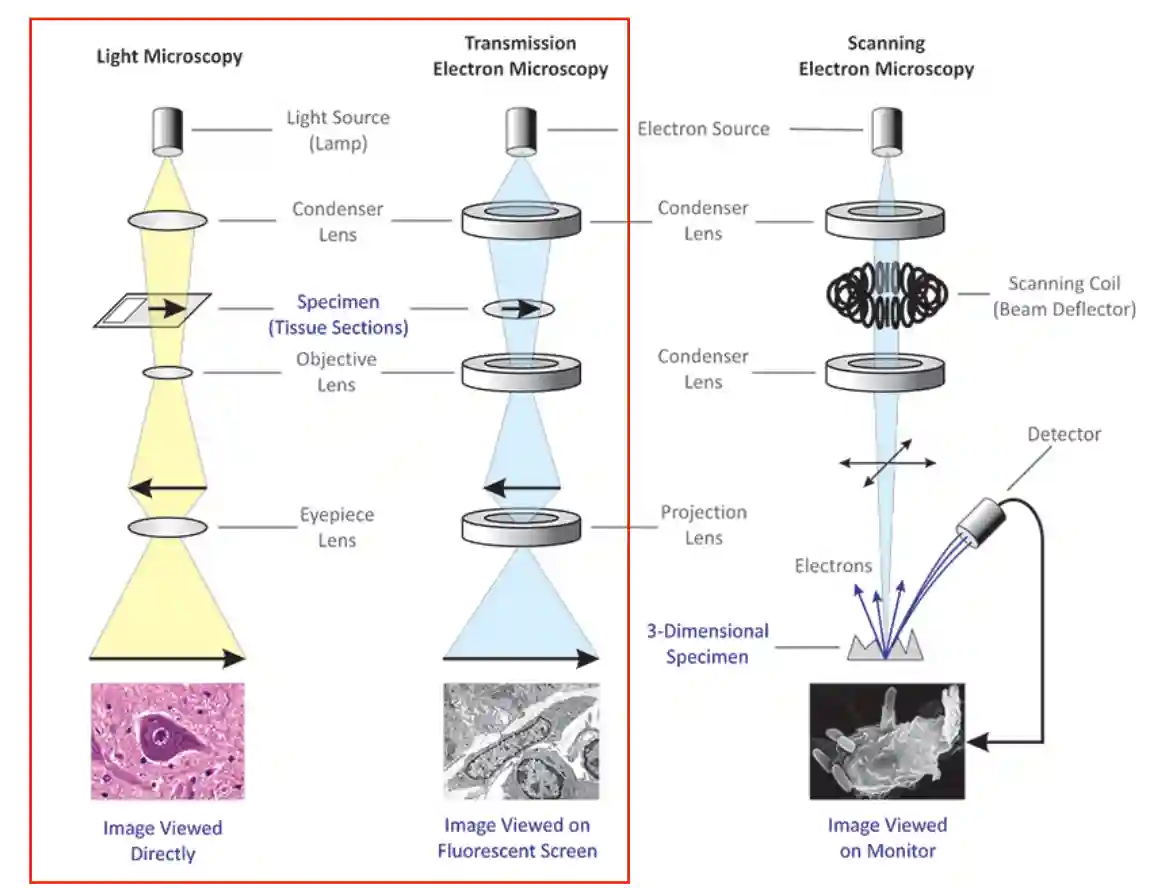
- LM -> 200nm
- TEM = Think transparency: electrons go through → internal structure, ultra-high resolution. 0.1-1 nm
- SEM = Think surface: electrons scan across → surface shape & composition. ~1-10nm
- Both are limited by sample prep complexity and vacuum requirements.
Types of lenses
Condenser
- Location: Just under the specimen stage.
- Role: Focuses light from the lamp onto the specimen → makes the illumination bright and even.
- Analogy: Like adjusting a flashlight so the beam spreads evenly over what you’re looking at.
Objective Lens
- Location: Closest to the specimen (the rotating lenses right above the slide).
- Role: This is the main magnifying lens. It gathers light from the specimen and creates a real, enlarged image inside the microscope.
- Magnification levels: Often 4×, 10×, 40×, 100×.
- Analogy: Like a zoom lens on a camera — the real workhorse of magnification.
Eyepiece
-
Location: The lens you look through at the top of the microscope.
-
Role: Magnifies the real image from the objective lens again, producing the final image that your eye sees.
-
Magnification level: Usually 10×.
-
Analogy: Like looking through binoculars to enlarge what the camera (objective) already captured.
-
Condenser = lights up the stage
-
Objective = magnifies the specimen’s image
-
Eyepiece = magnifies again for your eye
Comparison EM vs LM
One cubic millimeter would take thousands of hours. Now we can mimic human segmentation process, and we can build volumetric segmentation.
| Feature | Electron Microscopes | Light Microscopes |
|---|---|---|
| Maximum resolution | $0.5 \text{nm}$ | $200 \text{nm}$ |
| Useful magnification | Up to $250,000\times$ in TEM, $100,000\times$ in SEM | Around $1000\times$ ($1500\times$ at best) |
| Wavelength | $1.0 \text{nm}$ | Between $400-700 \text{nm}$ |
| Image Details | Highly detailed images, and even 3D surface imaging. | See reasonable detail, with true colours. |
| Applications/Specimens | Can see organelles of cells, bacteria and even viruses. | Good for small organisms, invertebrates and whole cells. |
| Feature | Light Microscopy | TEM | SEM |
|---|---|---|---|
| Resolution | ~200 nm | ~0.1 nm | ~1–10 nm |
| Live imaging | ✅ Possible | ❌ Impossible | ❌ Impossible |
| Color | ✅ Yes | ❌ No (grayscale) | ❌ No (grayscale) |
| Surface detail | ❌ Limited | ❌ Mostly internal | ✅ Excellent |
| Internal detail | ⚠ Limited | ✅ Excellent | ❌ Mostly surface |
| Sample prep complexity | Low | Very high | Medium |
| Imaging medium | Air or liquid | High vacuum | High vacuum |
| ! Example of scanning electron microscopy image, you can see the vesicles, the synaptic cleft and similar values. | |||
| In this setting, there is a big problem segmenting the single neurons and identifying what is valid or not. Now we can use machine learning methods to do the segmentation parts. |
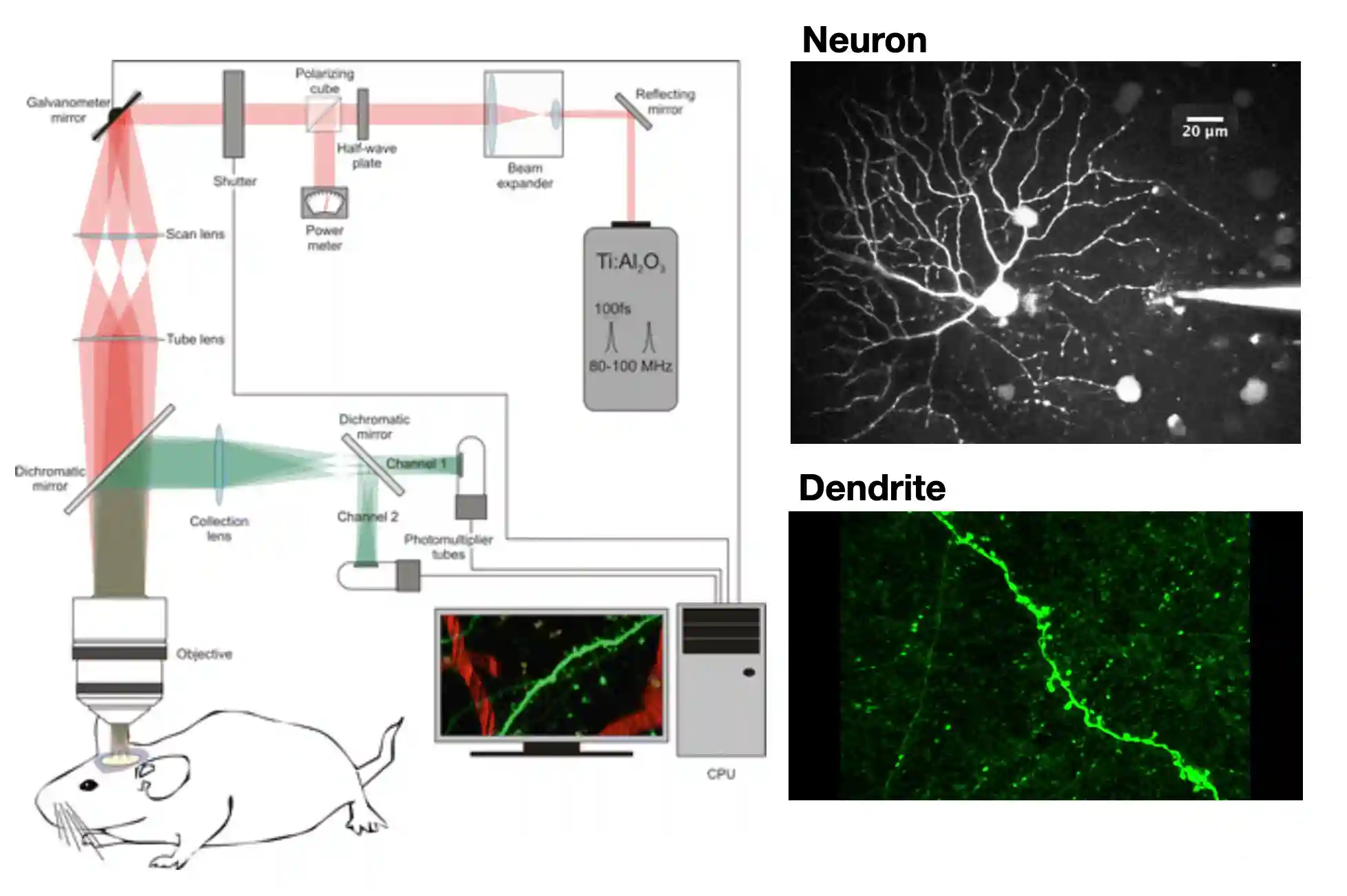
Fluorescence Microscope
We have a dichroic mirror The specimen shines in green light when you send some blue light to the specimen, which is then projected back to the camera lens.
Lower energy light is emitted. or emit more photons (super high density of photons in specific space). Red light is less scattered, due to higher wavelength, so it is a little better. This is why it is called two photon microscope, this is localized exitation, which means you get very crisp images.
! we need focused beams if we want to excite using lower wavelength sources We have 20$\mu m$, we don’t have neural overlapping, we can use Deep Learning to detect the neurons. Neuro finder challenge for example.
Two-Photon is nicer since the wavelength is smaller it:
- Scatters less: ~1.5mm! deep tissue imaging
- Less energy: so it does not do much photo damage to the tissue (at least less).
- But it has to be very much focused on the objective to create nice images.
GPT NOTES:
- Excitation source
- Intense light (mercury/xenon arc lamp, LEDs, or lasers) floods the sample at the excitation wavelength.
- Excitation filter
- Blocks all but the desired excitation wavelength from reaching the sample.
- Fluorophore absorption
- Target molecules in the sample absorb the excitation light and enter an excited electronic state.
- Emission
- As the fluorophores return to the ground state, they emit photons at the emission wavelength.
- Dichroic mirror
- Reflects the excitation wavelength toward the sample but lets the longer-wavelength emission light pass through to the detector.
- Emission filter
- Blocks any residual excitation light so only fluorescence reaches the detector/eyepiece.
Genetic Editing for Fluorescence Microscopy
A promoter is a region of DNA that initiates transcription of a particular gene (a promoter is a DNA sequence that turns the gene ‘on’). Promoters are located near the transcription start sites of genes, on the same strand and upstream on the DNA.
A reporter gene (often simply reporter) is a gene that researchers attach to a regulatory sequence of another gene of interest. The reporter is only expressed in those cells that express the gene. Certain genes are chosen as reporters because the characteristics they confer are easily identified and measured, or because they are selectable markers (e.g. such as green fluorescent protein, GFP).
Two Photon Microscopy
Two photon is very focused, I know excitation is just on that part of the light I am focused on.
Lightsheet microscope
You substitute first the layers of the sample with transpared molecules.
Then with this special type of microscope you can have nanometer resolution
- You illuminate only the plane you’re imaging — not the whole sample — which massively reduces photobleaching and speeds up imaging.
- The illumination and detection paths are perpendicular:
- One objective lens sends in a thin laser sheet (illumination axis).
- A second objective lens collects emitted fluorescence from the side (detection axis).
It is some sort of laser slicing thing.
General Microscopy Types
Superresolution Microscopy
You excite parts of die molecule (sparse manner), hopefully different, many times, and then combine the signals you get from the different images.
This was a light microscopy enhancement, which allows you to get high resolution. They won the nobel prize for this idea. The disadvantage is that it is slow, and cannot be done in vivo, because you need many many images to get the final image.
There are two main techniques for superresolution microscopy:
- STED (Stimulated Emission Depletion)
- First, excite fluorophores with a laser spot.
- Then, hit the same spot with a donut-shaped depletion beam that forces fluorophores in the periphery back to the ground state via stimulated emission.
- Only the tiny center region emits → effective resolution down to ~20 nm.
- SIM (Structured Illumination Microscopy)
- Illuminate the sample with a known interference pattern (grids or stripes).
- The moiré effect between the pattern and fine structures shifts high-frequency information into a range you can detect.
- Multiple patterned images at different angles are computationally reconstructed into a higher-resolution image (~100 nm lateral).
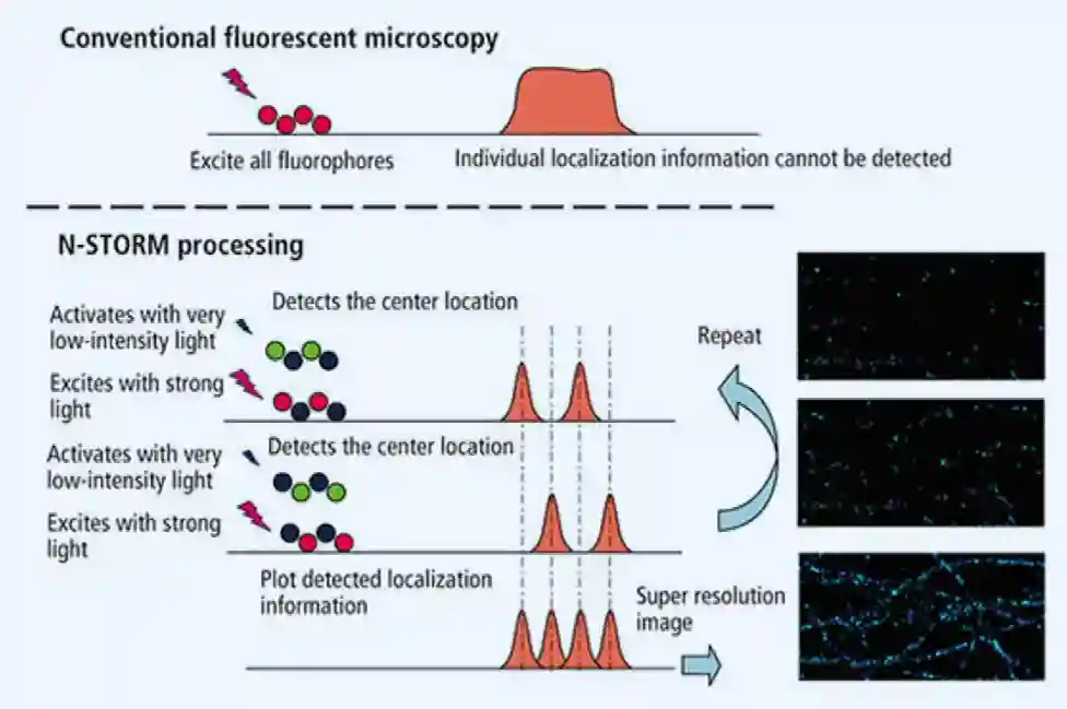
In the class we learned about STORM:
- Special fluorophores
- Uses dyes (often cyanine-based) that can be switched between a fluorescent (“on”) and a dark (“off”) state, either by specific wavelengths of light or by chemical environment.
- Sparse activation
- Only a random, sparse subset of fluorophores is switched on at any given moment.
- Because they’re far apart, their images don’t overlap — each appears as an isolated blurry spot (the point spread function, PSF).
- Localization
- For each spot, fit the PSF with a Gaussian to determine the emitter’s center with nanometer precision (often <20 nm accuracy).
- Switch off and repeat
- Turn those emitters off, switch on another random subset, and repeat thousands of times.
- Reconstruction
- Combine all localized points from all cycles into one composite super-resolution image.
The problem is that it is very slow, needs some high intensity lights and can damage cells.
Tetrode Recordings
Record spikes on 4 nearby contacts, detect events, extract multi-channel waveform features, cluster in 4-channel space, then validate with refractory/quality metrics—yielding isolated single-unit activity from a local population.
Functional Microscopy
This entails living cells (Calcium and Voltage images), and functional fluorescence indicators. You need to be fast, not like super-resolution one (slow imaging technique). Calcium is proxy of neural spiking, the nice thing is that we can see this in vivo.
We use very tiny microscopes, and get a movie out of that, and use this to detect the blinks. Usually it is terabytes of data.
Advantages of in Vivo
Voltage imaging -> something in the neurons that can be processed, meaning signal that can be received and made signal for. Another nice thing is that we can extract neuron firing voltage parts from image data. (microscopes create huge datasets).
Change in amplitude is linear with respect of the number of spikes, so I can kind of count the number of spikes in a zone. One of the downsides is that we are biased towards in vivo neurons. If a neuron never fires during our data gathering, then it is not good. for this. The important thing is that calcium is proxy of neural activity.
Synthetic Calcium Indicators
When calcium binds with BAPTA molecule, this changes shape, and can be detected. Nowadays we use GCamP6 protein (new indicator), which can create some nice images. Chemical dyes (e.g., Fura-2, Fluo-4) can be loaded into cells.
We can extract data of the activation of the Neural images using calcium in vivo functional imaging. In calcium imaging we leverage a dye could be synthetic or genetic dye (expressed by the neuron itself), when we have a spike, we have intercellular calcium and can be detected
General approach in extracting information
1.General Methods for cell extraction from Calcium Imaging Data- The PCA/ICA approach.- The Constrained Nonnegative Metrics Factorisation (CNMF) Approach2. Extracting Neuronal Signals from Multi-electrode recordings.- Filtering and defining signal features.- Clustering of cellular signals.3. Basics of Neuronal Population Analysis- Supervised and unsupervised extraction of population components- Decoding variables from neuronal population signals
Extracting Neural ROIs
At the time this paper was published, around 2010 the neural extraction was manual, so it was very important to find a manner to extract it automatically. One problem is to have overlapping ROIs
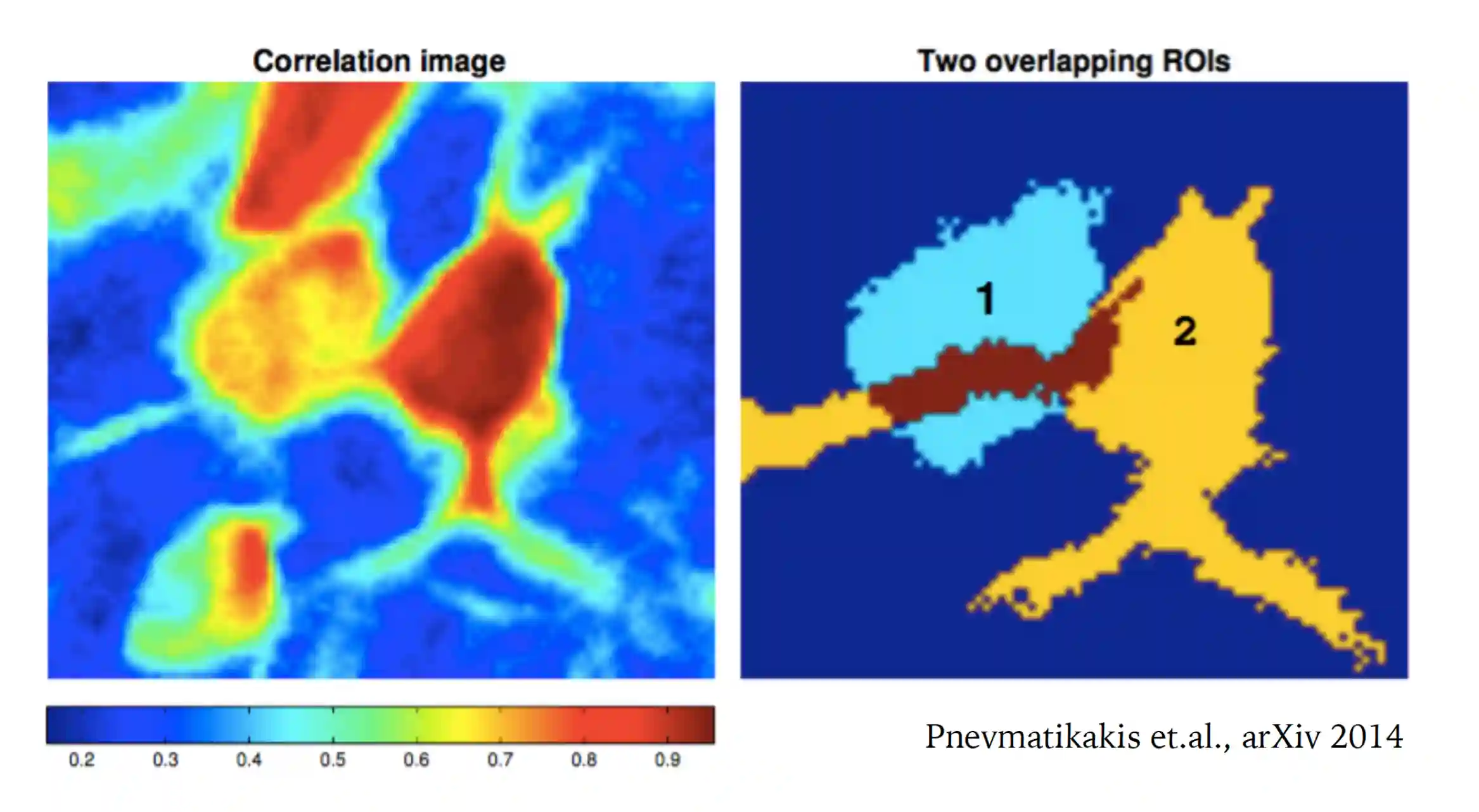 In miniscope imaging this is a big problem.
Since the ROI will detects some signal even if some signal is from the neighbours.
They have created **subtractive ROIs**, to get the difference between background and other things (we can catch contamination signals around).
In miniscope imaging this is a big problem.
Since the ROI will detects some signal even if some signal is from the neighbours.
They have created **subtractive ROIs**, to get the difference between background and other things (we can catch contamination signals around).
Decomposition of the neurons
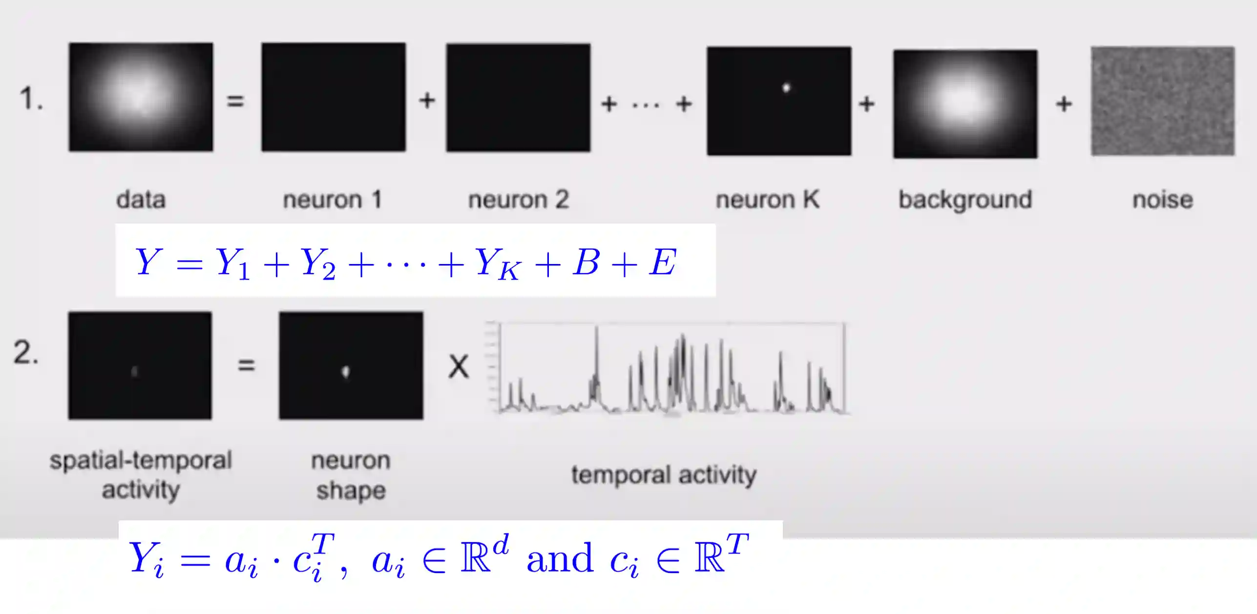 $$
Y = AC + B +E
$$
$$
Y = AC + B +E
$$We need to find $A$ and $C$ mainly. Quality of extraction depends on the quality of the contraints.
$A$ are the spatial footprints of our neurons. $C$ are the spatial components. $B$ is the background activity $E$ is the noise.
PCA/ICA
See Principal Component Analysis.
Neuron shapes and temporal components are spatially and temporally indipendent.
We want to get the principal components right.
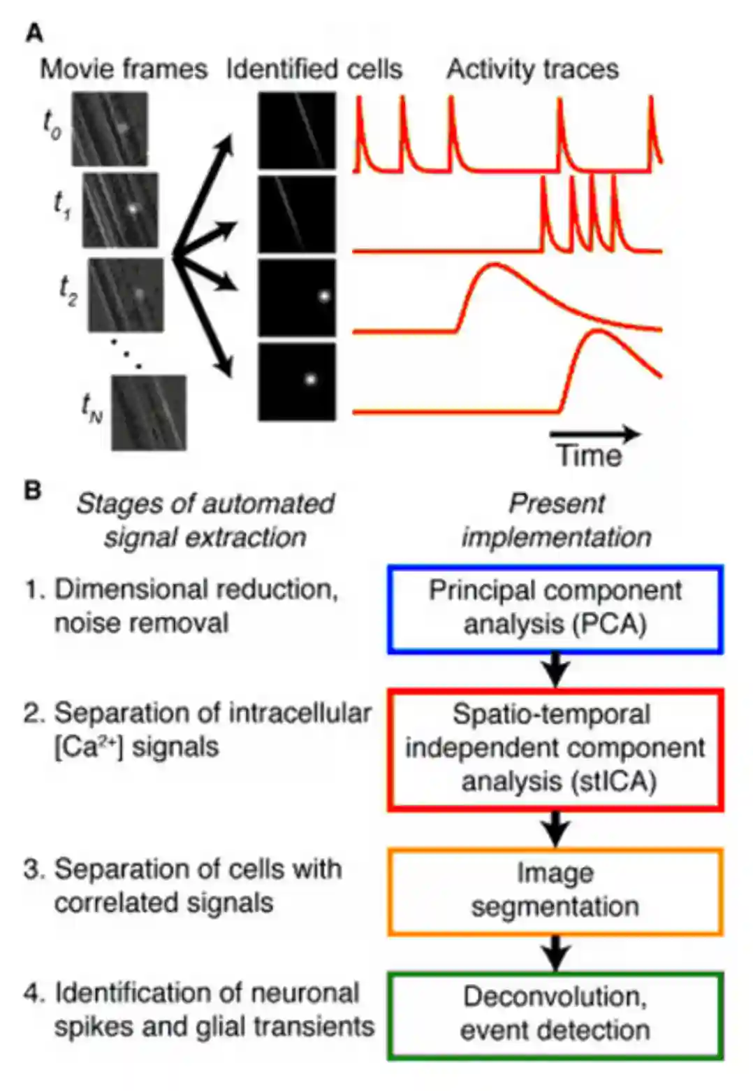
We want to find new statistically independent parts. The problem is that if regions are close, we get a small contamination of the signals. Sometimes we see negative activation due to removing activity in the zones.
Filters that induce maximum decorrelation sometimes is not feasible, since some neurons can be correlated. We wanted to have statistical independence in the neurons. ROIs for minimum correlation could be not a wanted notion.
Constrained Nonnegative Matrix Factorization
CNMF is a general framework for simultaneously denoising, deconvolving and demixing calcium imaging data.
We assume sparse spiking. Spatial and temporal components are all non negative.
$$ c_{i}(t) = \sum_{j = 1}^{p} \gamma_{j}^{(i)}c_{i}(t - j) + s_{j}(t) $$Where $s_{i}$ is the spiking signal.
Defining background in CNMF
The background fluctuation at each pixel can be represented as a linear combination of its neighboring pixels’ fluctuations.
We need to learn a weight matrix, how much one pixel influences its neighbour. We can recover fluctuations in this manner, but in simulated data.
The optimization objective
We model it as a linear optimization problem, so you can use Lagrange Multipliers
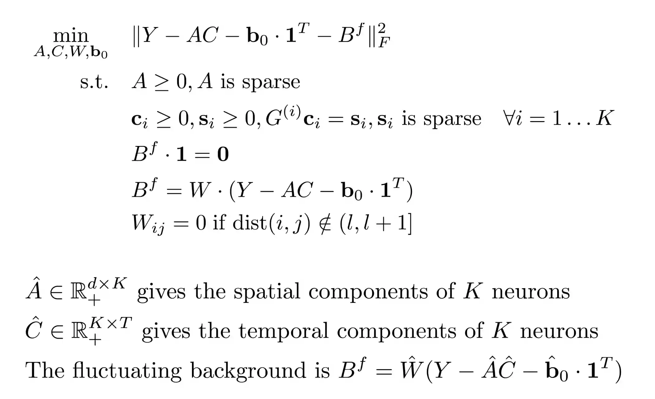
The technique then becomes a pipeline, since we need some $A, C, B$ estimates from the beginning.
We don’t see neighbour influence anymore
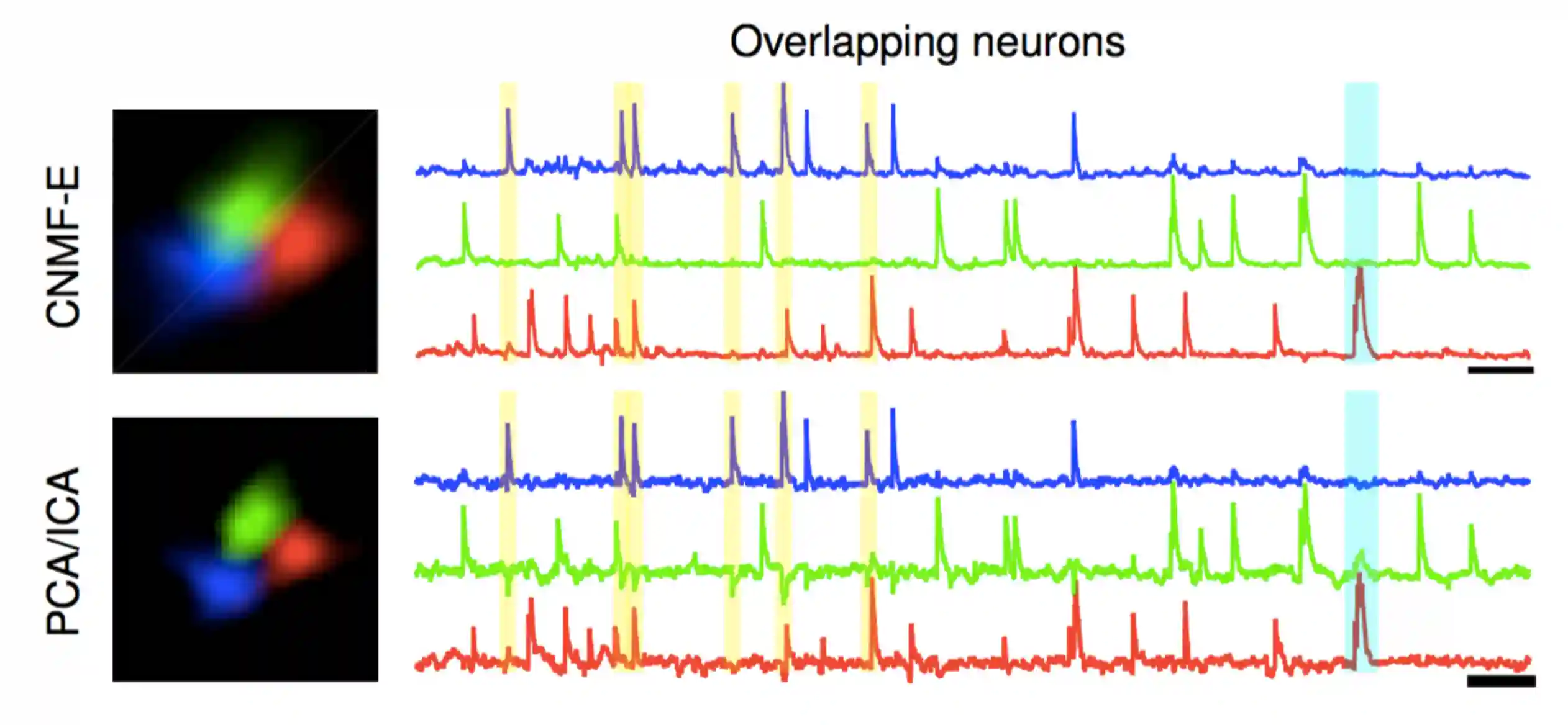

We don't have the problem of the negative values
Sorting pipeline
Some spikes have a very very small signal, they are very difficult to classify. Often we don’t have a nice profile, so we just cluster them together. We have thresholding mechanisms to do spike detection.
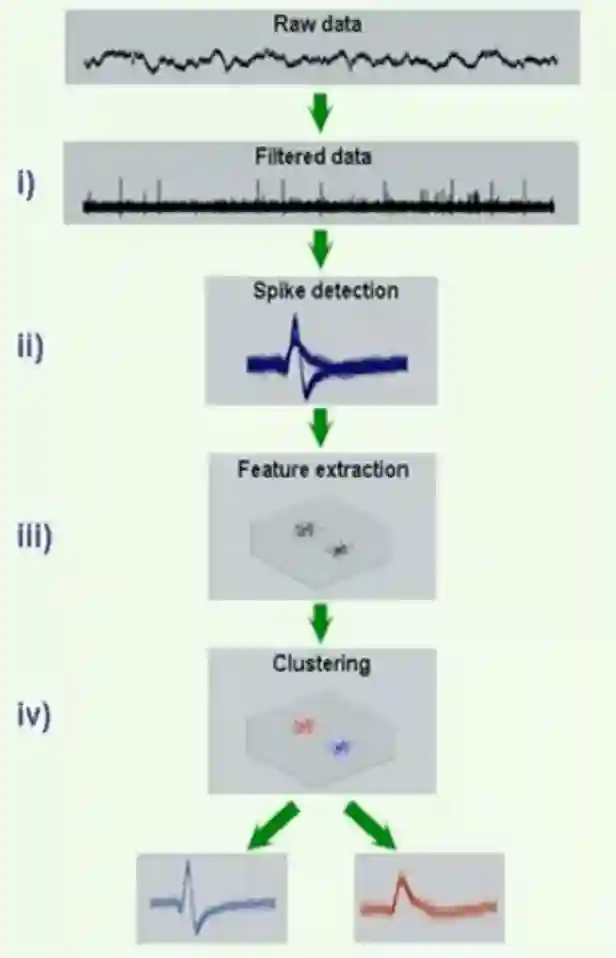
Filtering with Features
We have standard bandpass filtering 300-400: 4000-7000
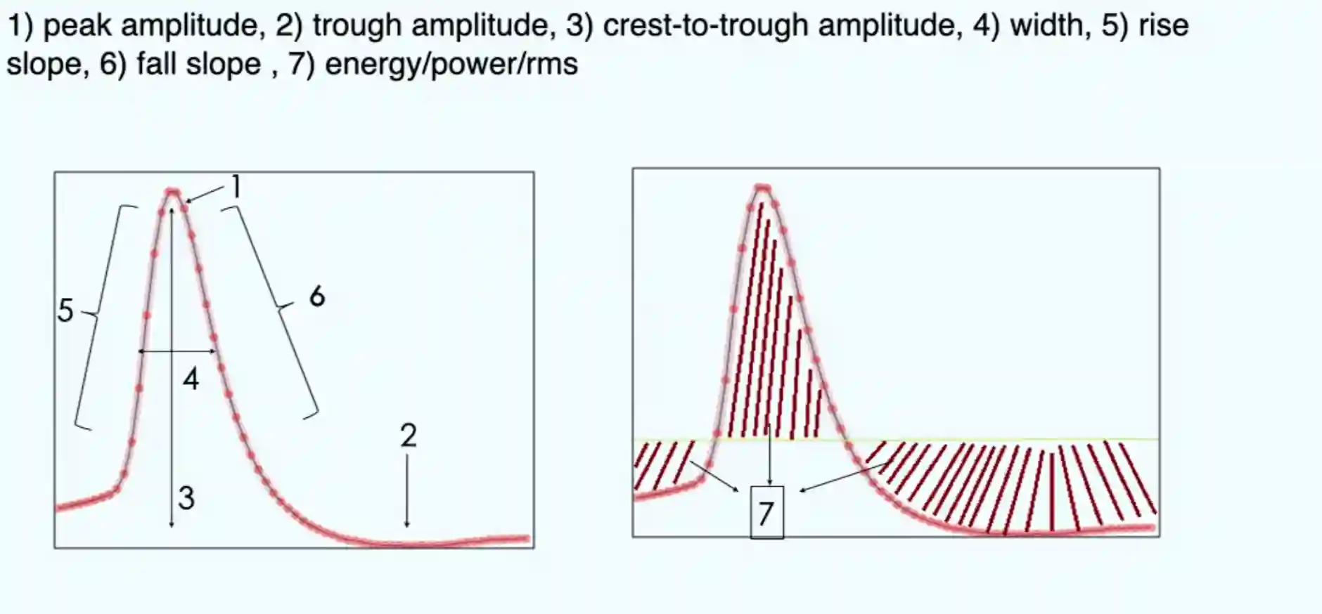
Then we can cut out a window around the spike, and that is our spike function. And we can take out features like:
- Peak amplitude
- Trough amplitude
- Crest to trough amplitude
- Width
- Rise slope
- Fall slope
One way is to use PCA to reduce it to few features and then use that. And this representation is nice for visual clustering of the type of spikes that we have.
Then we have many wavelets to chose from to model our neron activation.
Discrete Wavelet Transform
We use Discrete Wavelet transform with many convolutions. We know how much each wavelet is in the spike in this manner. It learns some coefficients to apply to the recorded data. Perhaps you can view this also as some kind of compression. Then we can sort by choosing the coefficients for higher variance.
Often this clustering part is done by humans after we have a good compression. We like to group population of neurons for some reason. I can do some sort of threshold analysis with that. This is called population decoder how the activation of a group of neurons move when activated. The decoder can tell you for example the position of a mouse by looking at grid maps of a in vivo recording for mices! You can use this only decoder when the variable of interest is related to your stuff. 89m 05.05.2025 video.
- Shuffled decoder comparisons are nice
Confounding variables for Neuron Imaging
- Neuron bursting: Spikes that occur in rapid succession (bursts) often have different waveforms than isolated spikes, potentially confusing spike-sorting algorithms or waveform-based analyses.
- Waveform overlaps of near-synchronous spikes: When multiple neurons fire nearly simultaneously, their extracellular waveforms can overlap, making it difficult to separate or identify individual neurons.
- Back-propagation of dendritic action potentials: These are action potentials traveling from the soma back into the dendrites. They can generate electrical signals that may be misinterpreted as separate spike events.
- Electrode drift over time: Physical movement of the electrode relative to the neuron (or vice versa) can cause changes in recorded waveforms, leading to incorrect clustering or loss of signal continuity.
- Bio-physiological differences across brain regions (CA1 vs. Cortex): Different brain regions can have different neuron types, morphologies, and firing properties, which may influence waveform shape and other features—limiting generalization across datasets.