An historical perspective

The origins of motion capture

One of the earliest starts of motion capturing is the famous horse in 1878 in motion “video”. This was the start of all the modern cameras. One of the earliest human body motion capture was in military for moving efficiency purposes in 1883. This website has many historical resources on the topic. The problem is still a problem in modern times. If we want to create models to mimic humans, it surely could be nice to understand how humans move and think. This is the general line of though of this line of research.

Human motion capture

One interesting experiment is that humans seem to automatically group dots that move together. It is research from many years ago, in Johansoon. Ten or twelve dots were enough for humans to have enough contextual information to have it make sense. This was the most important point of that research.

Problems in Human motion capture

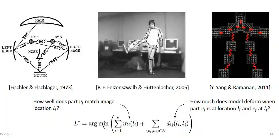
Following this idea, one interesting approach could be estimating 2D points from human images. The problems is taking into account for

• Plane rotations (head in different orientations)
• Scaling
• Perspectives
• Aspect ratio of different humans
• Intra-category variation (e.g. masked faces, particular faces with helmets, they should still be considered human faces) This idea first started with modelling with pictorial structures, like rectangles and things similar to that to model human faces. At the time, they didn’t have much data, and it was very difficult to extract those images. One of the earliest breakthroughs was from 2017 Cat et al. paper.

Early Models: Mass Spring and Pictorial Structures

Take cylinder primitives and fit to some representation. This was some physics based model to fit into some energy function. This inspired a lot of research. This was mainly a problem on representation. At the time it was very difficult to store images on the disk, there was not so much compute and data.

Modern Approaches

We know now how to extract features.

Earliest breakthroughs: Deep Features

This is called DeepPose. 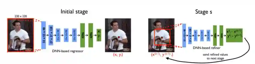Predicting heatmats was better than just predicting 2d points, so then people started to predict heatmaps for every single important joints, then you can sample from the joint. Then combined with the iterative approach they invented the next model.

You fit narrower and narrowerversions of the image to the model (stage modelling). After this, we went to regress for heatmaps, which was a better feature, meaning we have better results.

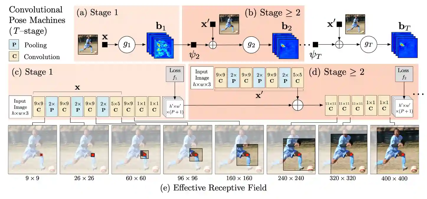
Convolutional Pose Machines

The network is able to look at the entire image after some iterations. Spatial correlations are taken into account here. So that deep models have big receptive field, while early stages are quite local, they add belief headmaps of the conditioned joints.

OpenPose and Part Affinity Fields

The use convolutional pose machines with iterative refinement and another branch with part affinity fields, to help with the association problem. This is a bottom-up approach, since we are feeding the whole image, without any preprocessing with that. The problem is that maybe we have many predictions for a single arm, and you need to join them together.

Part affinity fields:

• For every limb you create a unit vector that represents the moving direction of that limb. This helps with association strategies.
• Gives you direction of limbs that are then useful to solve the problem better, it looks very much like step by step solution in a supervised manner, closer to diffusions?

ViTPose

This is an example of a top-down approach (first use YOLO or similar things to have a good detection). There are many many other models that attempt to attack this section.

You get bounding boxes, and then fit the bounding boxes to a model that gives 2D detection, this helps you solve it without affinity fields, but needs 10x if there are 10 people in the image after you get a bounding box.

Usually 2D for humans, it is easy to annotate and check, but for 3D it is difficult to record and capture, we don’t have enough data for 3D, but we need to do it for this kind of problems, there are many papers that attacked this kind of zone.

Impactful models

Blanz and Vetter Face model

This is one of the classical statistical face models.. It is a statistical model that can be used to generate 3D human faces from 2D images. This example is still relevant today after 26 years.

Linear face representations

$$ S = \sum_{i = 1}^{m} a_{i} S_{i} $$

We want to have a general model that can generate all the faces.

This is desirable to have for:

• Simplicity in generation, you just need to find parameters starting from a fixed set of parameters.
• Generative model: we can generate new faces starting from the ones we have.

It is still hard problem, since just linear interpolation of pixels surely does not work.

Dense correspondence

We want point to point correspondence between parts of one face to another, i.e. a right eye corresponds to a right eye on the other face. One solution is adding one template face of fixed topology that helps in solving this representation. Yet this is some sort of a chicken and egg problem: having a morphable model would greatly help with the registration, but to build a morphable model we need to do registration.

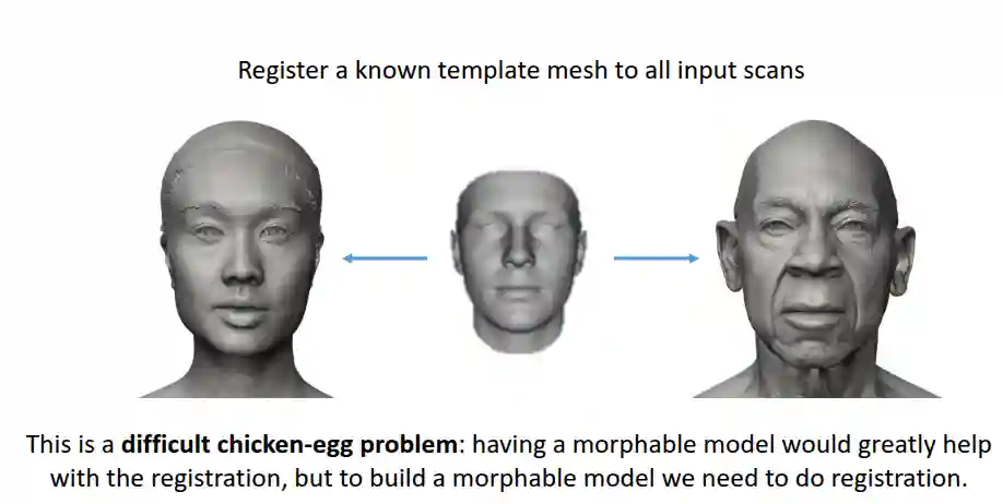
Use bootstrapping, the same idea we usually use to build compilers or RL Tabular Reinforcement Learning, Macchine Astratte, we have an algorithm that gives us a first model, and refine it iteratively.

Sensible Coefficients

How can you vary the coefficients to build some faces that do make sense? How to be sure that the produced face does indeed make sense? It was very difficult to get 3D data at the time, so the used Principal Component Analysis. You just assume that all shapes are in full correspondence, with a given topology, and compute the eigenvectors of the given faces dataset, it is exactly that. Given a set of $S_{i}$, you should be able to compute the principal components and take the eigenvectors.

$$ x = Uc = \sum_{i = 1}^{m} c_{i} \boldsymbol{u_{i}} = \sum_{i= 1}^{m} \left( U^{T}x_{i} \right) \boldsymbol{u_{i}} $$

You might also restrict this to a subset of the eigenvectors, to reduce the dimensionality of the problem. The geometry is high quality, and it is able to give 3D shapes from 2D images.

Statistical -> from data Shape -> from geometry priors.

SMPL

Published in SIGGRAPH Asia 2025. MPI in Tübingen, Germany, also called the SMPL Family.

SMPL (skinned, multi-person linear model) is a industry-standard built on linear-blend skinning (gives you a model that can be animated), used in both industry and research to model human bodies. It is a parametric model that can be used to generate 3D human bodies from 2D images. It is just an additive model, meaning it is simple, but with lots of parameters.

The model

$$ S = M(\theta, \beta) $$

Where $S$ is the 3D mesh and joints, $M$ is the SMPL model, $\theta$ is the pose parameters and $\beta$ is the shape parameters.

$$ \begin{align*} M(\theta, \beta) = W(T_{p}(\beta, \theta), J(\beta), \theta, \mathcal{W}) \\ T_{P}(\beta, \theta) = \bar{T} + B_{S}(\beta) + B_{P}(\theta) \end{align*} $$

Where:

• $W \in \mathbb{R}^{3N}$ outputs a mesh with $N$ vertices in 3D space
• $T_{P}(\beta, \theta)$ is the pose and shape parameters
• $J : \mathbb{R}^{\lvert \beta \rvert} \to \mathbb{R}^{3K}$ is the joint locations
• $\beta \in \mathbb{R}^{\lvert \beta \rvert}$ are the shape parameters, usually 10
• $\theta \in \mathbb{R}^{3K}$ are the pose parameters (joint angles for K joints)
• $\mathcal{W} \in \mathbb{R}^{K' \times 3N}$ is the skinning weights, with $K' \ll K$
• $\bar{T} \in \mathbb{R}^{3N}$ rest pose
• $B_{S}(\beta) \in \mathbb{R}^{3N}$ is the shape blend shapes
• $B_{P}(\theta) \in \mathbb{R}^{3N}$ is the pose blend shapes

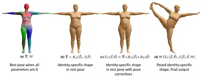
Rest Pose and Skinning Weights

The template was designed by an artist with 6.890 vertices and a segmentation part.

• The skinning weights (sparse matrix) $\mathcal{W}$ define how much every vertex is influenced by every joint under articulation (maximum of 4 joints)

Joints and Shapes

The shape blend shapes are linear offsets to represent the person’s shape. usually first 3 principal components. And it has different models for male and female.

$$ J(\beta) = \mathcal{J}(\bar{T} + B_{S}(\beta)) $$$$ B_{S}(\beta) = \sum_{i = 1}^{m} b_{i} \beta_{i} $$

and $b_{i}$ are the shape displacements learned with PCA from data.

Posing and Skinning

The pose assumes bone lengths are fixed, you can just do some rotations for every joint (rotations). So a pose is just a matrix of rotation information. SMPL uses angle-axis formulation around a normalized axis of rotation. Posing is determining the orientation of the joints.

$$ R_{k}^{\text{ global }} = R_{k}^{\text{ local }} R_{A(k)}^{\text{ global }} $$

Where $A(k)$ is the parent of joint $k$

From the rest position to posed space is named skinning, which is a rigid transformation. The details of the math is not important, so I will not report here.

$$ \sum_{k}w_{ji}G_{k}(\theta, J)t_{i} $$

Artifacts

LBS produces artifacts such as:

• Candy-wrapper artifact
• Collapsed joints (no good volume). You add corrections that make the shape look weird in unposed state, but ok in posed state. Artists usually add pose corrections, or you can learn it from the data.

We formulate the pose blend shapes as a linear function of the elements of the part rotation matrices.

Specifically, SMPL is represented by pose $\boldsymbol{\theta}$ and shape $\boldsymbol{\beta}$ parameters. Given blend skinning weights $w_{ki}$, rigid bone transformation $\mathbf{G}_k(\boldsymbol{\theta}, \mathbf{J}(\boldsymbol{\beta}))$, joint locations $\mathbf{J}$, shape correctives $s_i(\boldsymbol{\beta})$, and pose correctives $p_i(\boldsymbol{\theta})$ of a template mesh in rest pose, a deformed vertex $\mathbf{v}_i'$ is given by:

$$ \mathbf{v}_i' = \sum_k w_{ki} \mathbf{G}_k(\boldsymbol{\theta}, \mathbf{J}(\boldsymbol{\beta})) (\mathbf{v}_i + s_i(\boldsymbol{\beta}) + p_i(\boldsymbol{\theta})) $$

Pose Correctives

TODO, very strange formulation, difficult to understand…

Datasets and Registration

It starts with data gathering wit 3dMD scanners or similar scanning techniques that return point clouds. You need two datasets, shape (to get shape distributions), and pose datasets.

Then you use a shape dataset (high resolution scans of people in roughly the same pose) to learn the shape distribution in the population, of about 2k samples. There is a second dataset, the pose dataset, which is not publicly available for SMPL (Faust publishes some datasets). They put patterns on the skin to compare something I did not understood.

The high resolution scans are much higher resolution compared to possible templates. The poses can be complex, can have self-contact and lots of smooth areas. This is again some kind of a chicken and egg problem. Here they used co-registration where they solve it in a joint manner, they basically moved the shape into the scan to match.

Training the SMPL model

Initialization of the parameters

Our loss is the minimizing Euclidean surface reconstruction error. Our parameters are $\Phi = \left\{ \bar{T}, \mathcal{W}, \mathcal{J}, \mathcal{S}, \mathcal{P} \right\}$, with some regularization techniques to:

• Pose blend shapes $\mathcal{P}$ close to 0.
• Skinning weights $\mathcal{W}$ are initialized well (don’t know how close) and kept close (else it would probably not converge)
• Joint influence $\mathcal{J}$ is assumed to be local.

Pose Normalization

After, we train the T and S on shape dataset using PCA. and all shapes have the same pose normalization (we don’t want to learn differences due to pose).

optimization problem is formulated as:

$$ \hat{\mathbf{T}}_j^S = \underset{\hat{\mathbf{T}}}{\arg \min} \| W(\hat{\mathbf{T}} + B_P(\vec{\theta}_j; P), \mathcal{J}\hat{T}, \vec{\theta}_j, \mathcal{W}) - \mathbf{V}_j^S \|^2 $$

Where:

• $\hat{\mathbf{T}}_j^S$: The optimized template shape for the $j$-th registration.
• $\hat{\mathbf{T}}$: The template shape in T-Pose.
• $B_P(\vec{\theta}_j; P)$: A blend shape function that deforms the template based on pose parameters $\vec{\theta}_j$ and blend shape bases $P$, so that the only part that is unknown is the shape.
• $\mathbf{J}$: The Jacobian matrix relating pose parameters to vertex deformations.
• $\vec{\theta}_j$: The pose parameters for the $j$-th shape.
• $W$: Weights associated with the vertices or regions.
• $\mathbf{V}_j^S$: The $j$-th registered shape in the dataset.

PCA is computed on $\hat{T}_{j}^{S}$, which is the final shape.

The deformed template, representing the shape in a specific pose, is given by:

$$ \hat{\mathbf{T}} + B_P(\vec{\theta}_j; P) $$

The optimization aims to find the template shape $\hat{\mathbf{T}}$ that best fits all the registered shapes in the dataset after accounting for pose variations.

Other Applications

The SMPL family

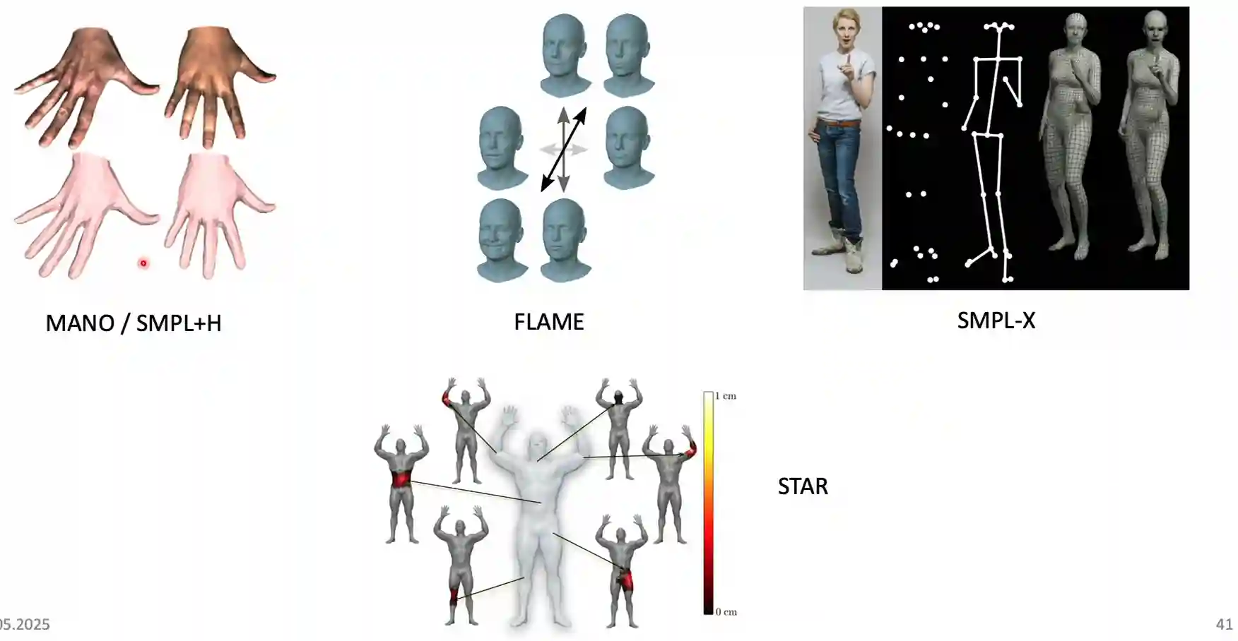
• SMPL+H adds hand joints, the standard does not have it.
• FLAME builds face models
• SMPL-X adds expressive (with facial expressions, models are more lifelike, they add articulations for the face)
• STAR adds more shape spaces, they can match more extreme shapes of the human body.
• SMPL-D (displacement) to add some shapes for the clothes.
  • It has some limitations (fixed resolution, but perhaps clothing needs more), this is some kind of a explicit modelling of the shape.

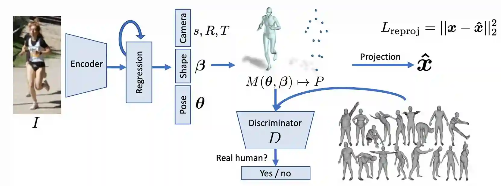
Human Mesh Recovery

See paper (Kanazawa et al. 2018). They use direct parameter regression to SMPL parmeters using Neural Networks, starting from single images, using 3D estimations. Statistical human body model to retrieve the correct model:

SMPLify

$$ \hat{\theta}, \hat{\beta} = \underset{\theta, \beta}{\arg \min} \| P(\theta, \beta) - P_{2D} \|^2 + \lambda_1 \| J(\theta, \beta) - J_{2D} \|^2 + \lambda_2 \| S(\theta, \beta) - S_{2D} \|^2 $$

Where:

• $\hat{\theta}$: The estimated pose parameters.
• $\hat{\beta}$: The estimated shape parameters.
• $P(\theta, \beta)$: The predicted 3D joint locations.
• $P_{2D}$: The observed 2D joint locations.
• $J(\theta, \beta)$: The predicted 3D joint locations.
• $J_{2D}$: The observed 2D joint locations.
• $S(\theta, \beta)$: The predicted 3D mesh.
• $S_{2D}$: The observed 2D mesh.
• $\lambda_1, \lambda_2$: Regularization parameters.

The idea is to add some regularization priors and try to match the 2D joints to the 3D joints. The problem is that the 2D joints are not always accurate, and the optimization can be difficult. One thing to note is that this paper was published in 2016.

Learned Gradient Descent

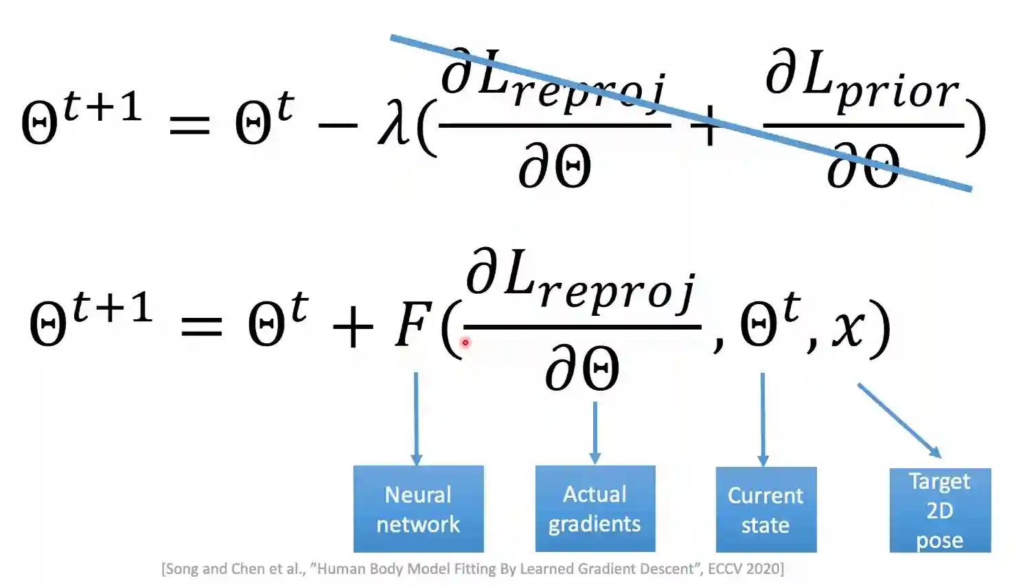
They show this provides much faster convergence, published in 2020. The problem was that the above descent was handcrafted, in this way you are using some differential network to estimate the difference, which is somewhat close to the ideas in Normalizing Flows for continuous ODE (see (Chen et al. 2019)).

They show this technique is much faster to converge compared to SMPLify.

Fitting IMU measurements

IMU are Inertial Measurement Units, which are used to measure acceleration and angular velocity. They can be used to fit the SMPL model to the IMU measurements. So that you can learn some actions.

You need a cost function for the orientation, and use that to regress to SMPL parameters and check the 3D pose of the human model.

Modelling Clothing

This lab proposed to add some modifications of the shape to model clothing. Problem is that the quality is fixed, something which is not always what we want. This is why sometimes implicit representations are better (see Advanced 3D Representations).

Modifying shapes is some form of an explicit representation.

References

[1] Kanazawa et al. “End-to-End Recovery of Human Shape and Pose” IEEE 2018

[2] Chen et al. “Neural Ordinary Differential Equations” arXiv preprint arXiv:1806.07366 2019