Transformers, introduced in NLP language translation in (Vaswani et al. 2017), are one of the cornerstones of modern deep learning. For this reason, it is quite important to understand how they are done.
Introduction to Transformers
Transformers are called in this manner because they transform the input data space into another with the same dimensionality.
The goal of the transformation is that the new space will have a richer internal representation that is better suited to solving downstream tasks. (Bishop & Bishop 2024)
General characteristics
One major advantage of transformers is that transfer learning is very effective, so that a transformer model can be trained on a large body of data and then the trained model can be applied to many downstream tasks using some form of fine-tuning.
Moreover, the transformer is especially well suited to massively parallel processing hardware such as graphical processing units, or GPUs, allowing exceptionally large neural network language models having of the order of a trillion (1012 ) parameters to be trained in reason- able time
A powerful property of transformers is that we do not have to design a new neural network architecture to handle a mix of different data types but instead can simply combine the data variables into a joint set of tokens.
Introduction to the structure
Transformers are just repeated blocks of attention layers, norms, MLP, followed by a final softmax on the final MLP layer, and preceded by a encoding layer. The first encoding layer has to embed some information about the original structure:
- Semantic information about the input
- Positional information about the input. Then we use the transformer blocks to process the input and get the final embedding layer.
Positional encoding
We need to keep positional information about the contents.
two randomly chosen uncorrelated vectors tend to be nearly orthogonal in spaces of high dimensionality, indicating that the network is able to process the token identity information and the position information relatively separately.
Binary positional encoding
This is just a simple idea to encode the information about the position of the tokens.
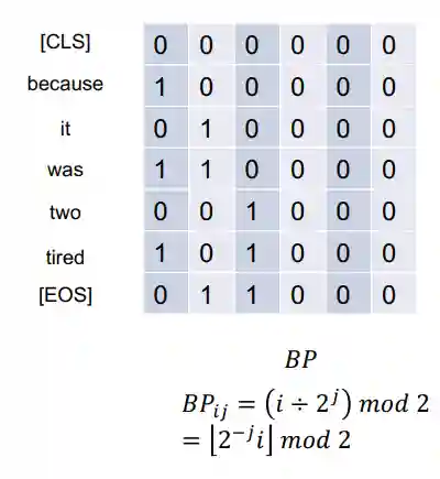
The above can be generalized with a periodic function (mod 2 equivalent but continuous) . A simple way is using and functions. But we would like a manner to encode the relative position between one token and another.
Sin and Cos positional encoding
You just put and then the positional encoding of a token and
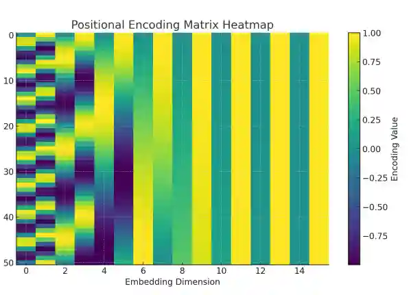
It's not clear why we need to interleave them.
Th: High dimensional unit vectors are almost always orthogonal
This theorem states that given , and we have that it is highly probable that . For a small epsilon. This is not exactly a formal proof (we haven't formalized the idea of highly probable)., but it gives an idea about why does it work. We will say that the expected product will be 0.
Proof To prove that two random high-dimensional vectors are nearly orthonormal, consider the following steps:
Step 1: Define the Vectors
Let be two independent random vectors with entries sampled i.i.d. from . Normalize them to unit length:
where .
Step 2: Compute the Dot Product
The dot product is . By linearity of expectation:
Step 3: Variance of the Dot Product
The variance is key to concentration. For normalized vectors:
Using independence and properties of unit vectors:
Thus, .
Step 4: Concentration via Chebyshev’s Inequality
For any :
As , this probability vanishes. Hence, in probability.
Step 5: Conclusion
Since and are unit vectors and their dot product concentrates around 0, they are nearly orthonormal in high dimensions. Specifically, for large , with high probability:
and their norms are exactly 1. This demonstrates the concentration of measure phenomenon in high-dimensional spaces.
Final Answer
Two random high-dimensional unit vectors are nearly orthonormal because their dot product concentrates around zero with variance , ensuring near-orthogonality, while their norms are exactly 1.
Two random high-dimensional unit vectors are nearly orthonormal with probability approaching 1 as dimension increases
Another fact: Concatenation is similar to addition: https://chatgpt.com/share/3bc87143-006a-4821-807e-5a35b06ec4da
Building the embeddings
Usually, the embeddings for each vector are backpropagated during training.
In Pytorch, you would use nn.Embedding. In this manner, each token is assigned a vector of size embedding chosen by the designer of the architecture.
This value is then initialized, and every index of the vector is a learnable parameter.
Attention
First introduced in (Bahdanau et al. 2014) in the context of translation.
Whereas standard networks multiply activations by fixed weights, here the activations are multiplied by the data-dependent attention coefficients.
Soft attention in which we use continuous variables to measure the degree of match between queries and keys and we then use these variables to weight the influence of the value vectors on the outputs.
Its main objective is to identify useful previous information.
The desiderata
We have said that transformers transform a set of data points into another with the same dimensionality. Attention is one important part of the architecture. To have richer representation space, we need each entry of the new vector to be a linear combination of the input. Plus, we need two properties for the attention coefficients:
- They should be positive or null (you pay some attention, or none, it doesn't make sense to have negative attention!)
- It should be limited (e.g. their sum should be 1), we choose one so that we don't make the variance of the input explode.
The intuition
Attention is an architecture used in Transformers to encode a soft version of dictionaries. In the context of text classification, the main intuition is giving a certain weight of some tokens, probably contextually more important, and less than others. If we have a query, which is something we would like to know about the text, then we try to match it with a key and the relative value. The softness of attention prevents us to say: "if the key doesn't match just return error", instead, it returns a linear combination of possible values, accordingly weighted by the rescaled keys.
Intuitively in the text context, attention models how much the value of one token influences another, directionally.
On the Asymmetricity
For example, we might expect that ‘chisel’ should be strongly associ- ated with ‘tool’ since every chisel is a tool, whereas ‘tool’ should only be weakly associated with ‘chisel’ because there are many other kinds of tools besides chis- els.
Asymmetric matrices have a higher relation representation capacity as we see from the above example. This motivates a different matrix for queries keys and values.
Self attention
Compared to a conventional neural network, the signal paths have multiplicative relations between activation values. Whereas standard networks multiply activations by fixed weights, here the activations are multiplied by the data-dependent attention coefficients.
Usually it is called self-attention when everything we want is just trying to change the values of the with a value. This value is called attention weight.
In standard attention based architectures the self-attention layer is computed as follows.
We have a set of weights , , of dimensions , and . Where is the batch size, is the latent size. Then, we say is a attention weight and we will have
And after you have computed the weights, you just apply it to the scaled values:
Apply this over all batches in a parallel manner.
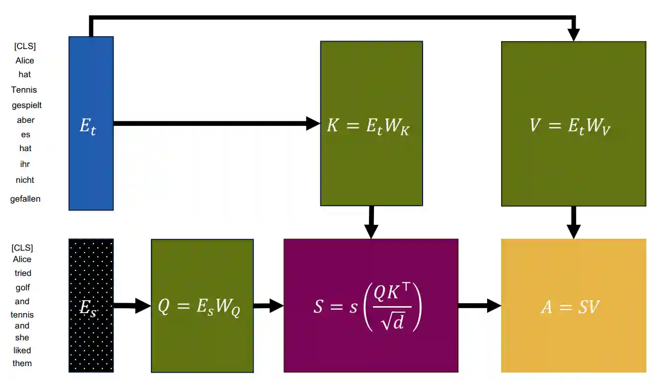
This image summarizes the main points of the attention mechanism.

Summarizes the main points of the attention mechanism
Why do we rescale? This is to keep the variance of the output the same as the input! If we assume that Q and K are normally distributed with variance 1 and mean 0, we are summing random variables with mean 0 and variance 1, then it's variance is (it's a quick exercise), dividing by keeps the variance unitary. In this manner, the numbers do not explode. See (Bishop & Bishop 2024).
The Cost of Attention
It is ,, we say it has a quadratic complexity:
- Similarity operation is quite heavy.
Cross-attention
In translation settings, we would like to add a context to the attention, meaning the key and query input values are different.
Causal-attention
This is also called the masked attention. In this case, we would like prevent the model to attend to tokens into the future. The intuition is easy: we just set the upper triangle to 0. We just set it to minus infinity.
The Architecture
Adding the embeddings
Since the positional embeddings are somewhat statistically independent from the token embeddings, both embeddings are somewhat orthogonal. Hence, the addition still preserves information about the two vectors. Since most of the operations done in an attention mechanism are linear. The final embedding is somewhat the addition of the result of the operations applied to both the positional and the token embeddings.
The whole architecture
This is the classical image by (Vaswani et al. 2017).
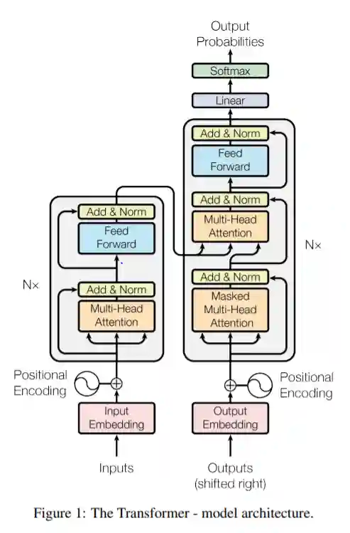
Which are just a lot of blocks concatenated with each other. In this case, the encoder and decoder are explicit.
Why GPT
- Performance: they are good at solving tasks
- Scalable: highly parallelizable architecture, good for training.
- They are able to model long range dependencies.
Visual Transformers
TODO
They also used masked autoencoders training, in a manner similar to how Bert is trained.
Applications
We will cover some very specific applications, clearly the main area of application is language modelling, with the currently famous GPT, Geminit etc models. We list here some of the relevant papers that were cited in the courses.
In Computer Vision
The main model applied here is the Vision Transformer.
ViT Pose
They use a ViT encoder and then a heatmap head (task specific) to decode pose information, they show better performance than previous state of the art
Sapiens
Many heads -> segmentation, depth, normal mesh, they could all be extracted from video image.
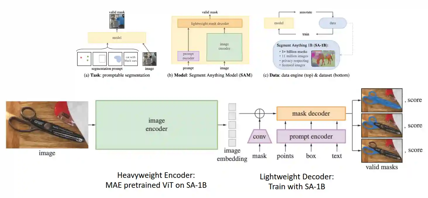
Segment Anything
Segmentation is the basis of everything in computer vision. This is a segmentation model that allows for different input modalities (also text for example). This model was from meta, and it was quite famous.
Multi-Modal
CLIP Model
We want to be able to produce image from caption and caption from image. So this is just some joint pretraining of captioned images, and it is able to do it well. Uses cosine similarity to do it.
One nice thing is using caption to classify the image, also better compared to some specific image classification methods.
DINOv2
CLIP models are limited by its training dataset, that needs pairs of images and texts. DINOv2 provides some features: it is self-distillation with no features. But here we don't have a teacher network -> idea to build it from past iterations of the student. Using DINO works better with other self-supervised methods, and even better to some supervised methods, probably it creates better features.
4M: Massively multimodal Masked Modeling
They basically project everything into a common embedding space:
- For text they use wordpiece
- For images they use VQ-VAE (see Autoencoders)
- For bounding boxes they use sequential prediction, similar to pix2seq. Then they train a single masked model to predict all the modalities.
DreamBooth
It is customized text-to-image generation. TODO: add more...
Zero-1-to-3: Finetune diffusion models with 3D data
Control camera perspective to generate some different views.
![[Transformers-20250530182641772.webp|Image from the website]]
SiTH
But does not work well for humans. Solved with Sith. SiTH: they do human mesh reconstruction to predict mesh, and then flip it to have the back image of the human, in this way the can produce consistent back views
References
[1] Vaswani et al. “Attention Is All You Need” arXiv preprint arXiv:1706.03762 2017
[2] Bishop & Bishop “Deep Learning: Foundations and Concepts” Springer International Publishing 2024
[3] Bahdanau et al. “Neural Machine Translation by Jointly Learning to Align and Translate” arXiv preprint arXiv:1409.0473 2014