On Autoregressivity
The main idea of autoregressivity is to use previous prediction to predict the next state.
The Autoregressive property
Autoregressive models model a joint distribution of aleatoric variables by assuming a chain rule like decomposition:
If we assume independence between the variables, we don't need many variables to model it , but this assumption is too strong. If we just use a tabular approach, we'll have a combinatorial explosion: we will have about possible states (if we assume the aleatoric variables are binary, and we are creating a table for each intermediate variable).
Fully Visible Belief Networks
This model attempts to solve the combinatorial explosion of previous auto-regressive setting, by modelling the next state as a bernoullian parameterized by some function:
If the parameters are different, this model just needs around parameters, where parameterizes
This is the idea of fully visible belief networks in the image below:
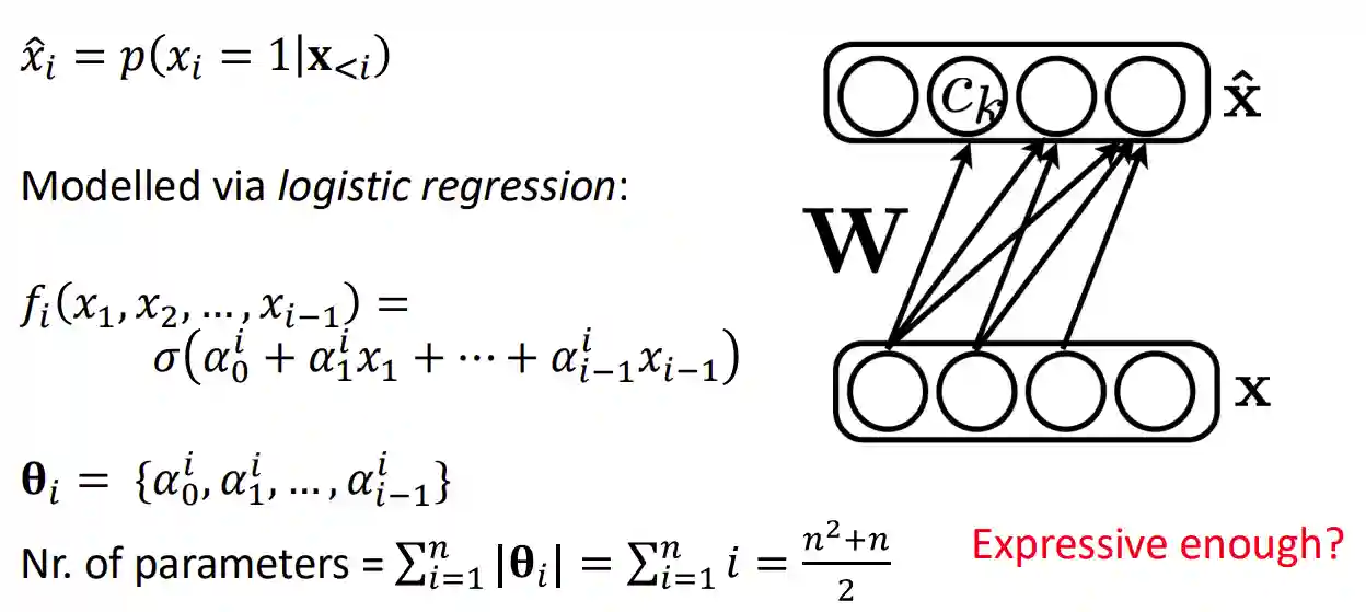
One of the main drawbacks of this model is the simplicity, which means probably it cannot encode many different functions. And heavy dependence on ordering (not all problems are text-like autoregressive).
Neural Autoregressive Density Estimation
These are other lecture notes: here, or see paper (Larochelle & Murray 2011). Here they add a number of hidden states to the model, which makes the model more expressive. This is the idea behind the Neural Autoregressive Density Estimation.
They leverage the probability product rule and a weight sharing scheme inspired from restricted Boltzmann machines, to yield an estimator that is both tractable and has good generalization performance.
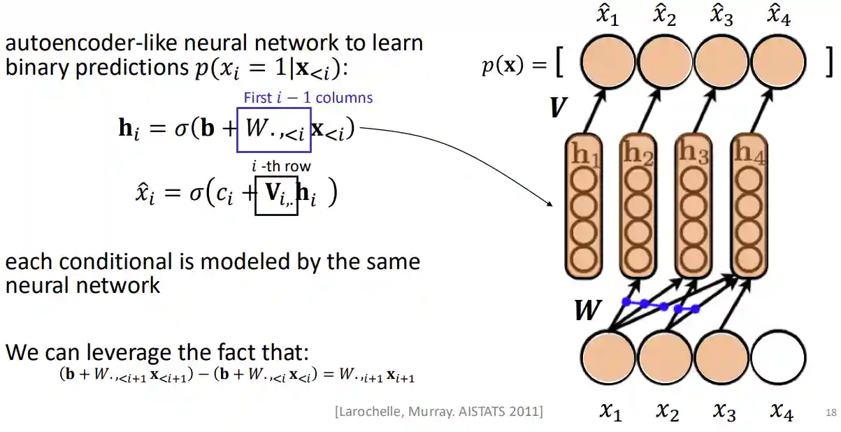 The number of parameters in this model is just instead of for the previous model. We have that where is the number of items and the feature vector length, and , and to have a prediction
And computing starting from the step before is also quite efficient. The is different for each timestamp.
The number of parameters in this model is just instead of for the previous model. We have that where is the number of items and the feature vector length, and , and to have a prediction
And computing starting from the step before is also quite efficient. The is different for each timestamp.
Training is done by maximizing log-likelihood.
The computations are efficient, and the model is also resistant to the ordering of the inputs!
An alternative view of NADE is as an autoencoder that has been wired such that its output can be used to assign probabilities to observations in a valid way.
There are many extension works around.
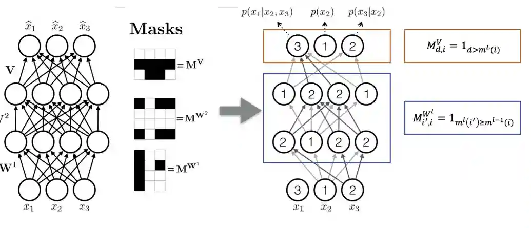
Masked Autoencoder Distribution Estimator
The idea is to Constrain Autoencoder such that output can be used as conditionals, see (Germain et al. 2015). What they have done is to mask out every computational path between and the ones with indexes above them.
- Training has the same complexity as regular autoencoders
- Criterion is Negative Log Likelihood for binary
- Computing is just a matter of performing a forward pass
- Sampling however requires forward passes
- In practice, very large hidden layers necessary, it makes it a little bit too large, probably it's because the neurons are quite restrained regarding their possible connections that they can have.
- Note: the mask for value and weights are different. But I don't know why.
The key is to use masks that are designed in such a way that the output is autoregressive for a given ordering of the inputs, i.e. that each input dimension is reconstructed solely from the dimensions preceding it.
I would say this is the idea preceding BERT (Devlin et al. 2019), basically they are able to model autoregressive things, by sampling some kind of ID, and putting connections only to the ones with ID above them.
The problem perhaps is that with this architecture, the neurons are quite limited? Meaning, they cannot express their full thing. The vertical part of the mas is the output, the input is on the horizontal part.
On Image and Audio
We can define a notion of order on images and audio, and then use autoregressive models to generate them. It depends on how you define the autoregressive property on images. (e.g. see image patches, and resolution pyramids).
PixelRNN
Model introduced in (van den Oord et al. 2016).
 So the idea here is very simple, just a RNN applied on images.
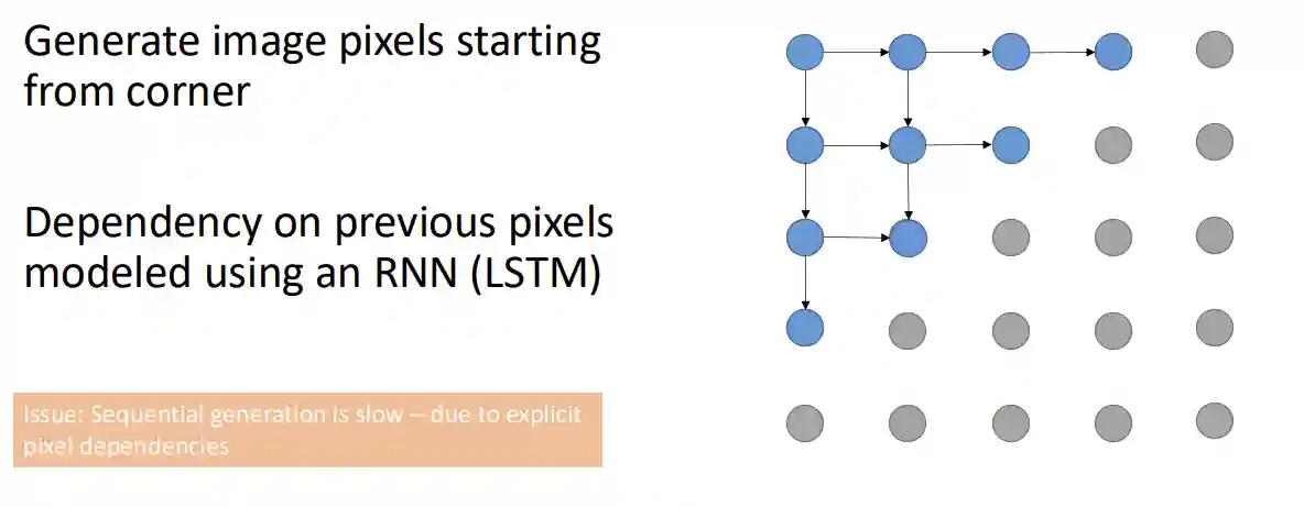
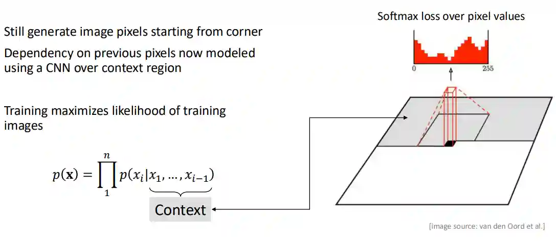
PixelCNN
This model was introuduced in the same paper as PixelRNNs.
They start to generate pixels from the top left corner and then continue to generate it using some receptive field of the pixel. This makes:
- Training efficient
- Parallelizable training, but not inference (and they showed the performance in accuracy is quite similar, so you gain in training).
This has similar quality compared to pixel RNN, but it is faster. But the generation is still sequential, which makes it slow.
A nice thing with these is that they had an explicit negative log likelihood to compare with old models.
WaveNet
It is an auto-regressive model for audio generation. It uses a stack of dilated temporal convolutions to generate audio (problem is much larger dimensionality compared to images). It can generate audio samples at a rate of 16kHz. It is also slow in generation. they use temporal causal networks to attempt to model long range dependencies.

We can observe here the effect of dilated convolutions on the receptive field of the model.
Transformers
See Transformers.
References
[1] Larochelle & Murray “The Neural Autoregressive Distribution Estimator” JMLR Workshop and Conference Proceedings 2011
[2] Germain et al. “MADE: Masked Autoencoder for Distribution Estimation” PMLR 2015
[3] Devlin et al. “BERT: Pre-training of Deep Bidirectional Transformers for Language Understanding” arXiv preprint arXiv:1810.04805 2019
[4] van den Oord et al. “Pixel Recurrent Neural Networks” PMLR 2016