Backpropagation is perhaps the most important algorithm of the 21st century. It is used everywhere in machine learning and is also connected to computing marginal distributions. This is why all machine learning scientists and data scientists should understand this algorithm very well. An important observation is that this algorithm is linear: the time complexity is the same as the forward pass. Derivatives are unexpectedly cheap to calculate. This took a lot of time to discover. See colah’s blog. Karpathy has a nice resource for this topic too!

A Brief History of Backpropagation

Backpropagation builds on some backbone ideas in mathematics and computer science.

• Building blocks of backpropagation go back a long time

  • The chain rule (Leibniz, 1676; L’Hôpital, 1696)
  • Dynamic Programming (DP, Bellman, 1957)
  • Minimisation of errors through gradient descent (Cauchy 1847, Hadamard, 1908)

• in the parameter space of complex, nonlinear, differentiable, multi-stage, NN-related systems (Kelley 1960; Bryson, 1961; Bryson and Denham, 1961; Pontryagin et al., 1961, …)

• Explicit, efficient error backpropagation (BP) in arbitrary, discrete, possibly sparsely connected, NN-like networks apparently was first described in 1970 by Finnish master student Seppo Linnainmaa

• One of the first NN-specific applications of efficient BP was described by Werbos (1982)

• Rumelhart, Hinton and William, 1986 significantly contributed to the popularization of BP for NNs as computers became faster. We also list this resource, it is a quite nice view on backpropagation as an optimization problem. But if you just study for the exams, probably this is not necessary.

The problem setting

We have a dataset $D$ with input-output pairs, we have a loss function $\mathcal{L}$ and we want to find this

$$ \min_{\theta} \sum_{(x, y) \in \mathcal{D}} \mathcal{L}(f(x ; \theta), y) $$

A common tool is gradient descent but we need to compute the gradients for this algorithm. The astounding fact is that the speed of computing the gradients is same as a forward pass. In optimization classes computing the gradients is given for granted, while the algorithm itself is not trivial.

In the old times people would calculate the gradients by hand for every parameter. We need automatic differentiation and we will explain here how does it work.

Automatic Differentiation

We will use a specific type of automatic differentiation, called reverse-mode. This is not all automatic because we need to know

• How to decompose the whole function in easy parts
• Need to know the differential of the simple primitive functions that we use compute the forward pass. We can summarize the whole thing with this theorem:

Reverse-mode automatic differentiation can compute the gradient of $f$ in the same time complexity as computing $f$

This will be a constructive theorem. First refresh some basis of analysis, see for example Limiti, Derivate, Hopital, Taylor, Peano, Calcolo differenziale, e Jacobians, and some notes about Computer Science i.e. Notazione Asintotica.

Hypergraph

TODO: see (Huang 2008) for discussion on hypergraphs in NLP.

Computational graphs 🟨

A composite function is a function composed by a series of (nonlinear) functions. Hypergraph is a graph that allows hyperedges, which is a edge that branches into more than one node, or two edges that merge into one, so it allows to have more than one source or more than one target, in normal graphs we only have single source and single targets for an edge. In the graph, the squares are hyperedges, the order of the input nodes usually matters (for example for the division operator).

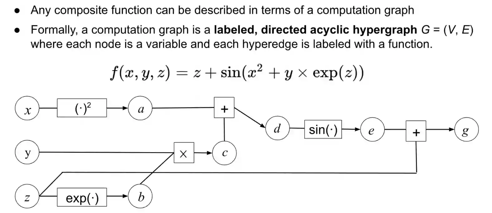
For example the $+$ is a hyper-edge with two parents. We need hyper edges because we need a kind of ordering.

It’s easy to see that we have an exponential number of paths in the computational graph when computing the derivative, because we need to account all possible paths where it can propagate!

$$ \frac{ \partial y }{ \partial x } = \sum_{p \in \mathcal{P(i, j)}} \prod_{(k, l) \in p} \frac{ \partial z_{l} }{ \partial z_{k} } $$

Meaning we need to find all paths from $i$ to $j$ and then use the chain rule to compute the gradient contribution for this path. And this algorithm is exponential in time complexity.

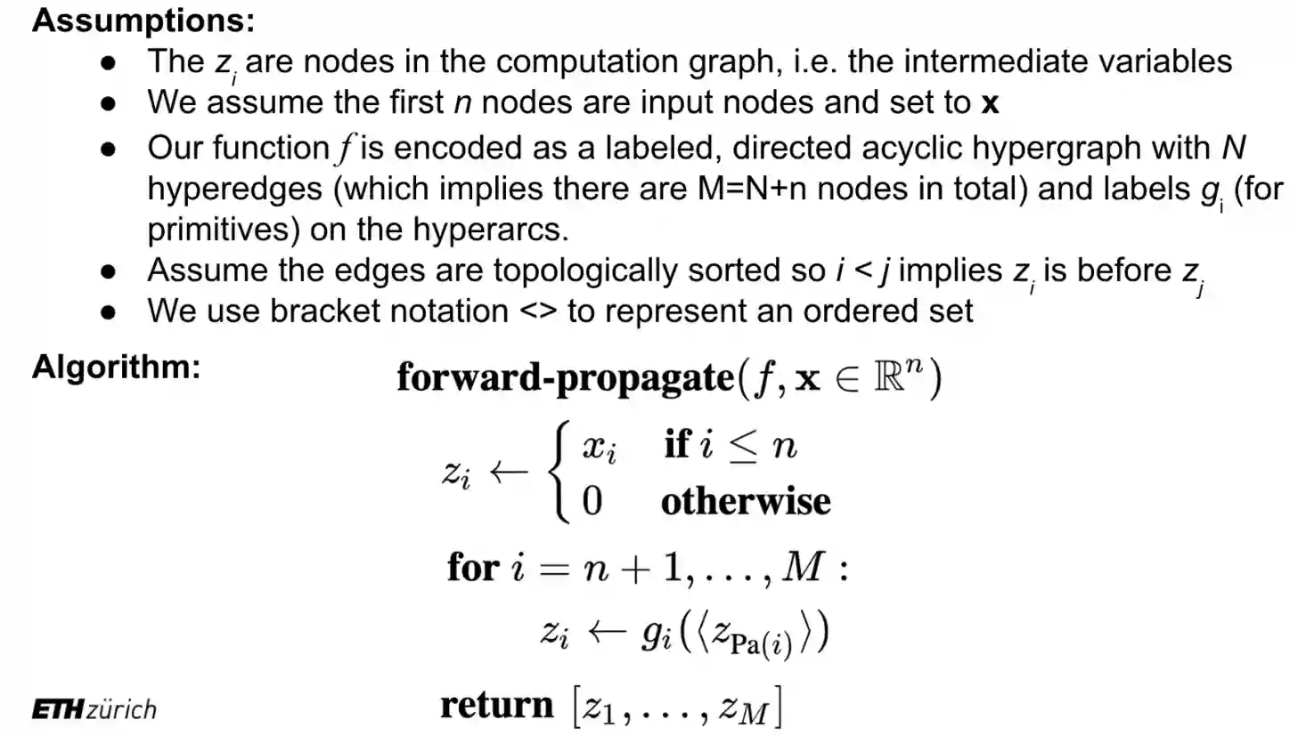
The forward pass 🟩

We can write the forward pass of this algorithm in the following way:

The backward pass 🟩–

The optimal accumulation problem is NP-hard. This problem has some similarities with the backward pass.

We just to the backward pass, this example is explanatory: 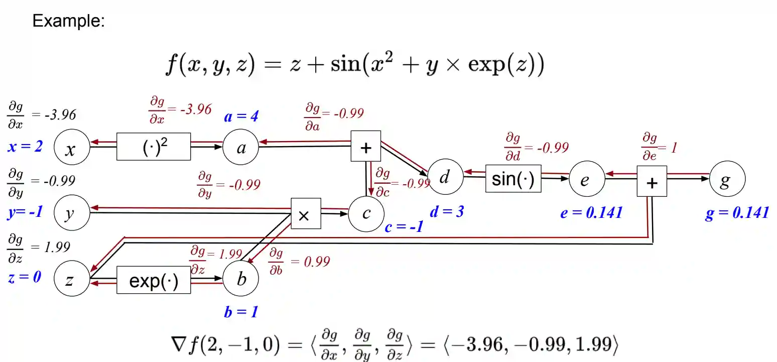You can see that the derivative of $g$ to intermediate point is stored when doing the backpropagation part, and this makes it easy to propagate back step by step.

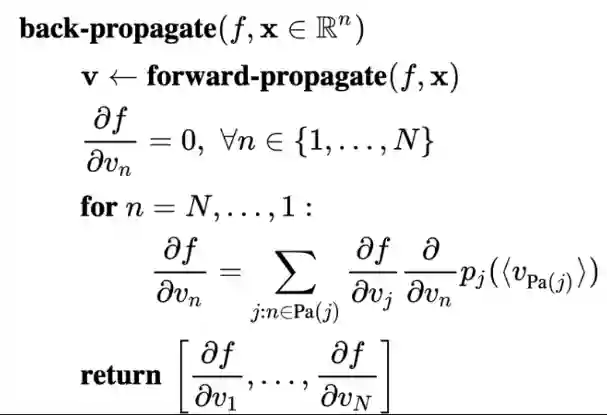
We can write the algorithm mathematically

Bauer Paths 🟨–

Bauer’s formula is a chain rule but for a graph! Given a function $f: \mathbb{R}^{n} \to \mathbb{R}^{m}$ for input $x_{j}$ and output $y_{j}$ we have that

$$ \frac{ \partial y_{i} }{ \partial x_{j} } = \sum_{p \in \mathcal{P}(j, i)} \prod_{(k, l) \in p} \frac{ \partial z_{l} }{ \partial z_{k} } $$

Where $\mathcal{P(j, i)}$ is the set of all paths from $j \to i$ and $(k, l)$ are the individual edges. Every path in this formula is called Bauer Path.

The following is an example: .

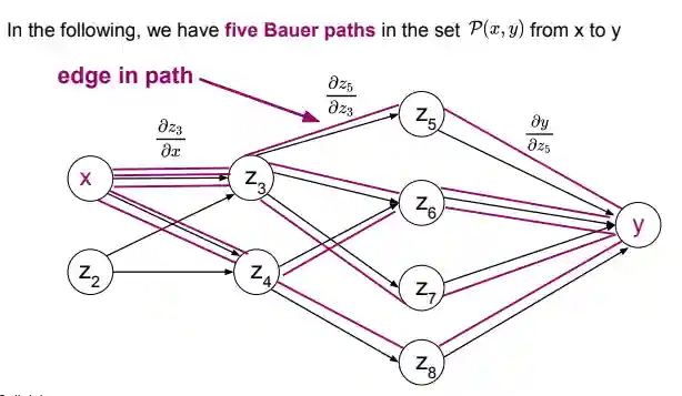We have many of the paths are re-used! This is also why dynamic programming is important at this stage. Weird but interesting thing is that there is a link between factoring polynomials and dynamic programming, but I did not understand why.

Types of Differentiation

There are other types of automatic differentiation. In this section we will briefly present two of the most known aside auto-grad.

Numerical differentiation 🟩

This is the form of differentiation that can treat the function actually as a black box, and you can prove bounds about this. You just try to compute the function many times with sensitivity analysis and assume the result is an approximation. The drawback is that this scales on the number of inputs, so it’s much more slower.

$$ \frac{ \partial f(x, y, z) }{ \partial z } \approx \frac{f(x, y, z + h) - f(x, y, z)}{h} $$

Symbolic differentiation 🟩-

This is what is done by engines like wolphram alpha, it computes the real derivative of the expression, but this is inefficient because in some cases there is repeated computation when the same expression compares in different parts. I don’t know how exactly is done by automatic differentiation, but probably you as a programmer need to write the function in some specific way.

Supplementary notes

With this notion of gradient flow, one can try to generalize this notion and create works like this (Du et al. 2023). Where the only thing needed is to have a semi-ring and then you can use the same algorithm for some interpretability analysis or similar.

A simple exercise

We will attempt to use backpropagation for the following function so that we can understand a little bit more about this algorithm:

$$ f(x, y, z, v) = \exp(y ^{-x} - \log(z)) + (y - z)^{2} \cdot \log(v) $$

Let’s try to calculate its symbolic gradient, that is $\nabla f$, so we need to calculate every partial derivative:

$$ \begin{array} \\ \frac{ \partial f }{ \partial x } = \exp(y^{-x} - \log(z)) \cdot e^{-x \log y} (-\log y) \\ \frac{ \partial f }{ \partial y } = \exp(y^{-x} - \log(z)) \cdot e^{-x \log y} (-x / y) + 2(y - z) \log(v) \\ \frac{ \partial f }{ \partial z } = \exp(y^{-x} - \log(z)) / (-z) - 2(y - z) \log(v) \\ \frac{ \partial f }{ \partial v } = 0 + \frac{(y - z)^{2}}{v} \end{array} $$

We can observe that with the symbolic method a lot of computation is repeated in the $\exp$ thing.

This is an example of the computational graph (forward in red and backward in blue, it has a small mistake when computing the backwards for the exponential function)

Check the original excalidraw here.

An algorithm for k-th order gradients

If we know the computational graph of a certain function, it becomes also easy to compute the k-th gradient. Let’s now consider the simple case of computing the hessian. We know that if $m$ is the number of edges in the computational graph, we need $m$ operations for the forward and $m$ operations for the backward, thus giving us $\mathcal{O}(m)$ complexity for computing the $\nabla f$. What about $\nabla^{2}f$? We notice that

$$ \nabla^{2}f = \begin{bmatrix} \nabla (e_{1}^{T} \nabla f(x)) \\ \vdots \\ \nabla (e_{n}^{T} \nabla f(x)) \end{bmatrix} $$

This is a handy relation, that could be extended also to the $k-th$ order case. We need $\mathcal{O(m)}$ operations to compute the gradient for a single component, we just unfold the computation graph (we take the last backward used for the gradient, as another forward component) and do the same for every component. This algorithm runs in $\mathcal{O(n \cdot m)}$. It’s easy to prove by induction that if we apply the same algorithm, in order to compute the $k$ order algorithm it will take $\mathcal{O}(n^{k - 1}m)$ time.

References

[1] Du et al. “Generalizing Backpropagation for Gradient-Based Interpretability” 2023

[2] Huang “Advanced Dynamic Programming in Semiring and Hypergraph Frameworks” Coling 2008 Organizing Committee 2008