Bayesian Linear Regression

We have a prior $p(\text{model})$, we have a posterior $p(\text{model}\mid \text{data})$, a likelihood $p(\text{data}\mid \text{model})$ and $p(\text{data})$ is called the evidence.

Classical Linear regression

Let's start with a classical regression. In this setting we need to estimate a model that is generated from this kind of data:

$$y=w^{T}x+\epsilon$$

Where $\epsilon \sim \mathcal{N}(0,{\sigma }_n^{2}I)$ and it's the irreducible noise, an error that cannot be eliminated by any model in the model class, this is also called aleatoric uncertainty. One could write this as follows: $y\sim \mathcal{N}(w^{T}x,{\sigma }_n^{2}I)$ and it's the exact same thing as the previous, so if we look for the MLE estimate now we get

$${\hat{w}}_{\text{MLE}}=\arg \underset{w\in {\mathbb{R}}^d}{\max }\sum _{i=1}^N\log p(y_i\mid x_i,w)=\arg \underset{w\in {\mathbb{R}}^d}{\min }(y-w^{T}x{)}^2$$

And this result is quite nice, because we just discovered that with this assumptions the best model for classical linear regression, the minimizer for the ordinary least squares problem, gives the same result with the maximum likelihood estimator.

One random note is that the complexity of computing linear regression is

$$\mathcal{O}(d^{2}N+d^3)$$

Where $d$ is the dimensionality of the input and $n$ the number of samples. Using the closed formula approach. Usually the Gradient Descent method might be a little faster. It costs $\mathcal{O}(nd)$ per iteration.

Ridge Regression

Before diving into this section, you should know Ridge Regression quite well.

Maximum a posteriori estimate leads to Ridge Regression

We assume a prior $p(w)=\mathcal{N}(0,{\sigma }_p^{2}I)$ (this is the special thing about Bayesian learning, which gives us confidence bounds, we choose Gaussians because of nice properties, see Gaussians and the Maximum Entropy Principle), and we also assume that $w$ is independent of the $x_{1:n}$, this further assumption acts as a regularization, as we will see briefly. The conditional likelihood is $p(y_{i:n}\mid w_i{x}_{i:n})={\prod }_{i=1}^{n}p(y_i\mid w_i{x}_i)$ so we assume that the $y_{i:n}$ are conditionally independent given $w_i{x}_{i:n}$. And we further assume that

$$p(y_i\mid w_i{x}_i)=\mathcal{N}(y_i;w^T{x}_i,{\sigma }_n^2)$$

Which is the same as saying that $y_i=w^T{x}_i+{\epsilon }_i$ where ${\epsilon }_i\sim \mathcal{N}(0,{\sigma }_n^2)$.

Now we can model the posterior:

$$p(w\mid x_{1:n},y_{1:n})=\frac{1}{z}p(w\mid x_{1:n})p(y_{1:n}\mid w_i,x_{1:n})$$

And $z=\int p(w)p(y_{1:n}\mid w_i,x_{1:n})dw$.

Now let's expand everything: we will have:

$$\frac{1}{z}\cdot \frac{1}{z_p}\exp \left(-\frac{1}{2{\sigma }_p^2}\Vert w{\Vert }_2^2\right)\cdot \frac{1}{z_l}\prod _{i=1}^n\exp \left(-\frac{1}{2{\sigma }_n^2}(y_i-w^T{x}_i{)}^2\right)$$

Let's call $z^{\prime }=z\cdot z_p\cdot z_l$ and now we have this:

$$=\frac{1}{z^{\prime }}\exp \left(-\left[\frac{1}{2{\sigma }_p^2}\Vert w{\Vert }_2^2+\frac{1}{2{\sigma }_n^2}\sum _{i=1}^n(y_i-w^T{x}_i{)}^2\right]\right)$$

Now we do Max. a posteriori (MAP) estimate for $\hat{w}$ and we get this:

$$\begin{array}{r}\hat{w}=\arg \underset{w}{\max }\log p(w\mid x_{1:n}{y}_{1:n})\\ \\ =\arg \underset{w}{\max }\log p(y_{1:n}\mid x_{1:n},w)+\log p(w)\\ =\arg \underset{w}{\min }\sum _{i=1}^k(y_i-w^T{x}_i{)}^2+\frac{{\sigma }_n^2}{{\sigma }_p^2}\Vert w{\Vert }_2^2\end{array}$$

Which we note is the same as Ridge regression with $\lambda =\frac{{\sigma }_n^2}{{\sigma }_p^2}$. So with those Gaussian assumptions we just go back to a standard regression case! Remember that if $\lambda =0$ we don't have basically a regularizer, if $\lambda$ is high we practically don't care much about the data (if noise is high we want to regularize, but if the prior variance is small we regularize more)

The MAP estimate simply collapses all mass of the posterior around its mode. This can be harmful when we are highly unsure about the best model, e.g., because we have observed insufficient data.

This why usually bayesian methods are preferred in other times.

And interesting observation is that one could derive the lasso regression if we assume the underlying distribution of $p(w)$ to be a Laplacian instead of a Gaussian. This should enable us to perform variable selection. But the lasso optimization is usually not derivable (computed using LARS or similars), and the form is not exactly nice. For completeness, we report it here anyways: The prior on the weights should be in this case

$$p(w)=\prod _{i=1}^d\frac{{\sigma }_p^2}{4{\sigma }_n^2}\exp \left(-\frac{{\sigma }_p^2}{2{\sigma }_n^2}|w_i|\right)$$

No clue how to derive it though. I took this from slide 12 here (you need eth credentials to access the resource).

Posterior is Gaussian

In theory this result is easy if you know what are The Exponential Family and see that Gaussian is a Conjugate prior of itself. We observe that we can rewrite the argument part of the exponent in the following equation to be a gaussian:

$$p(w\mid x_{1:n},y_{1:n})=\frac{1}{z^{\prime }}\exp \left(-\left[\frac{1}{2{\sigma }_p^2}\Vert w{\Vert }_2^2+\frac{1}{2{\sigma }_n^2}\sum _{i=1}^n(y_i-w^T{x}_i{)}^2\right]\right)$$

We can rewrite it as $(w-\bar{\mu }{)}^T\bar{\Sigma }(w-\bar{\mu })$ where

\begin{array} \\ \bar{\Sigma} = \left( \frac{1}{\sigma_{n}^{2}} X^{T}X + \frac{1}{\sigma_{p}^{2}}I \right)^{-1} = \sigma_{n}^{2}\left( X^{T}X + \frac{\sigma^{2}_{n}}{\sigma_{p}^{2}} I \right) ^{-1} \\ \bar{\mu} = \frac{1}{\sigma_{n}^{2}} \bar{\Sigma} X^{T}y = (X^{T}X + \lambda I)^{-1} X^{T}y \end{array}

Where $\lambda$ is as before, and this is the link with linear regression! This form is nice as it allows to have some confidence intervals over the parameters.

Inference

Inference in Bayesian Linear Regression

The main idea is to have predictions that are weighted by the probability of the model, so we write:

$$p(y^{\ast }\mid x^{\ast }{x}_{1:n}{y}_{1:n})=\int p(y^{\ast },w\mid x^{\ast },x_{1:n},y_{1:n})dw=\int p(y^{\ast }\mid w,x^{\ast })p(w\mid x_{1:n}{y}_{1:n})dw$$

We won't actually use this model for inference. In the case of Bayesian Linear regression we have a simpler case, which can be written as follows: We first used the sum rule, then we used product rule and independence assumption . Let's suppose $f^{\ast }=x^{\ast T}w$ so we use the multiplication of Gaussians with a constant ($x^{\ast }$) rule and get

$$p(f^{\ast }\mid x^{\ast },x_{1:n},y_{1:n})=\mathcal{N}(f^{\ast };{\bar{\mu }}^T{x}^{\ast },x^{\ast T}\bar{\Sigma }{x}^{\ast })$$

And assuming $y^{\ast }=f^{\ast }+\epsilon$ we have sum of Gaussian is Gaussian so we have

$$p(y^{\ast }\mid x^{\ast },x_{1:n},y_{1:n})=\int p(y^{\ast }\mid w,x^{\ast })p(w\mid x_{1:n}{y}_{1:n})dw=\mathcal{N}(y^{\ast };{\bar{\mu }}^T{x}^{\ast },x^{\ast T}\bar{\Sigma }{x}^{\ast }+{\sigma }_n^{2}I)$$

So compared to ridge regression, the Bayesian linear regression has a variance term that is added. Here we are using all possible models, weighted by their probability. Conceptually bayesian is better than MLE.

It is possible to see later with the law of total variance, the decomposition of the inference variance into epistemic and aleatoric variance.

Relation between BLR and Ridge Regression

Ridge regression can be viewed as approximating the full posterior by placing all mass on its mode (also other models can be seen similarly, one example is MLE, analyzed in Parametric Modeling).

So it's a nice approximation:

$$\begin{array}{r}p(y^{\ast }\mid x^{\ast },x_{1:n},y_{1:n})=\int p(y^{\ast }\mid w,x^{\ast })p(w\mid x_{1:n}{y}_{1:n})dw\\ \approx \int p(y^{\ast }\mid w,x^{\ast }){\delta }_{\hat{w}}(w)dw\\ =p(y^{\ast }\mid x^{\ast },\hat{w})\end{array}$$

Remember that for delta direct distribution we have

$$\mathbb{E}[f(x)]=\int f(x){\delta }_{x^{\prime }}(x)dx=f(x^{\prime })$$

Epistemic and aleatoric uncertainty

We now start a philosophical discussion on epistemic and aleatoric uncertainty.

• Epistemic uncertainty: Uncertainty about the model due to the lack of data
• Aleatoric uncertainty: Irreducible noise

The $x^{\ast T}\bar{\Sigma }{x}^{\ast }$ is the epistemic uncertainty about $f^{\ast }$ while the ${\sigma }_n^2$ factor is the noise/uncertainty about $y^{\ast }$ given $f^{\ast }$, meaning we need to change $f^{\ast }$, or hypothesis class if we want to lower this uncertainty I think (not sure though).

The law of total variance can give another intuition about the decomposition between epistemic and aleatoric uncertainty:

$$Var(y\mid x)=\text{ aleatoric }+\text{ epistemic }={\mathbb{E}}_{\theta }\left[{\text{Var}}_y(y\mid x,\theta )\right]+{\text{Var}}_{\theta }({\mathbb{E}}_y[y\mid x,\theta ])$$

Choosing hyper-parameters

We would like a manner to compute the values of ${\sigma }_n^2$ and ${\sigma }_p^2$. Covariance of the prior and variance of the noise need to be chosen before we can apply these methods. One way is just finding $\lambda =\frac{{\sigma }_n^2}{{\sigma }_p^2}$ with cross-validation, then estimate the variance from data and get the prior variance in this manner.

Then it's possible to have graphical models for bayesian linear regression.

Recursive bayesian updates

We want to incorporate the data we have today as future prior. The posterior we have today will be the prior of tomorrow. Let's suppose we have $p(w)$ prior and we have observations $y_{1:n}$ such that $p(y_{1:n}\mid w)={\prod }_{i=1}^{N}p(y_i\mid w)$ We can define some intermediate posteriors:

$$p^{(j)}(w):=p(w\mid y_{1:j}),p^{(0)}(w)=p(w)$$

If we have the posterior for the previous $j-1$ data points and now we have $y_j$, then we can compute the next prior (we used Bayes rule here and i.i.d. property of $y_i$):

$$p^{(j)}(w)=p(w\mid y_{1:j})=\frac{1}{z}p(w)\cdot p(y_1\mid w)\dots p(y_j\mid w)=\frac{1}{z}\left(z\cdot p^{(j-1)}(w)\right)p(y_j\mid w)=f(p^{(j-1)}(w),y_j)$$

So we would just need to integrate the new information given by $y_j$ and then use the previous knowledge. The recursive updates are also the reason why the Dirichlet is a nice prior for multinomials, see Dirichlet Processes.

Example: Bayesian Update for a Coin toss

We can see how the posterior changes with the number of coin flips. We will use a Beta prior for the Bernoulli likelihood, this is a conjugate prior so we can compute the posterior in closed form.

import numpy as np
import matplotlib.pyplot as plt
from scipy.stats import beta

# Initialize parameters for the Beta prior
alpha_prior = 1  # Prior "successes" (e.g., heads)
beta_prior = 1   # Prior "failures" (e.g., tails)

# Simulated coin flips (1 = heads, 0 = tails)
np.random.seed(42)  # For reproducibility
coin_flips = np.random.choice([0, 1], size=100, p=[0.7, 0.3])  # Unfair coin: 70% tails, 30% heads

# Function to plot the Beta distribution
def plot_beta(alpha, beta_val, flip_num):
    x = np.linspace(0, 1, 1000)
    y = beta.pdf(x, alpha, beta_val)
    plt.plot(x, y, label=f"After {flip_num} flips (α={alpha}, β={beta_val})")
    plt.xlabel("Probability of Heads (p)")
    plt.ylabel("Density")
    plt.title("Online Bayesian Update of Beta Distribution")
    plt.legend()

# Create a figure for the updates
plt.figure(figsize=(10, 6))

# Perform Bayesian updates after each coin flip
for i, flip in enumerate(coin_flips):
    # Update the Beta prior with the Bernoulli likelihood
    alpha_prior += flip  # Increment alpha if heads (flip=1)
    beta_prior += 1 - flip  # Increment beta if tails (flip=0)
    
    # Plot the updated distribution every few flips
    if i in {0, 4, 9, 19, 99}:  # Plot at these specific flips
        plot_beta(alpha_prior, beta_prior, i + 1)

# Show the final plot
plt.grid(alpha=0.3)
plt.show()

Online Bayesian regression

This section concerns in building a bayesian regression algorithm whose memory does not grow with the number of samples. It can be conceived as a filtering process, composed of two phased: conditioning (updating over the priors) and prediction.

We have discovered a manner to learn the best parameters for bayesian linear regression which is just this closed form:

$$p(w\mid X,y)=\mathcal{N}(w;(X^{T}X+{\sigma }_n^{2}I{)}^{-1}{X}^{T}y,({\sigma }_n^{-2}{X}^{T}X+I{)}^{-1})$$

Assuming ${\sigma }_p^2=1$.

Now we want to do online linear regression, assuming the data is coming one by one, we would like to update the corresponding matrices of interest, which are $X^{T}X$ and $X^{T}y$. So, let's say we are given some matrices

$$X^{(t)}=\left[\begin{array}{c}{x}_1^T\\ ⋮\\ x_t^T\end{array}\right]\in {\mathbb{R}}^{t\times d}{Y}^{(t)}=\left[\begin{array}{c}{y}_1\\ ⋮\\ y_t\end{array}\right]\in {\mathbb{R}}^{t\times 1}$$

We would like to efficiently compute $X^{(t+1)T}{X}^{(t+1)}$ and $X^{(t+1)T}{Y}^{(t+1)}$ assuming the known matrices above. The latter is easy to compute because:

$$X^{(t+1)T}{Y}^{(t+1)}=\sum _{i=1}^t{x}_i{y}_i+x_{t+1}{y}_{t+1}=X^{(t)}{Y}^{(t)}+x_{t+1}{y}_{t+1}$$

Now let's try to decompose the other product

$$X^{(t+1)T}{X}^{(t+1)}=\left(\begin{array}{c}{x}_1,\dots x_t\end{array}\right)\cdot \left(\begin{array}{c}{x}_1\\ ⋮\\ x_t\end{array}\right)=\sum _{i=1}^t{x}_i{x}_i^T+x_{t+1}{x}_{t+1}^T=X^{(t)T}{X}^{(t)}+x_{t+1}{x}_{t+1}^T$$

This allows to compute the parameters in a way that the memory requirement is constant and does not grow as $\mathcal{O}(t)$.

Another problem that we have is computing the inverse of $X^{T}X+{\sigma }_n^{2}I$ is very expensive, usually takes $\mathcal{O}(d^3)$ but we can do it in $\mathcal{O}(d^2)$ with the use of Woodbury Identities: If $A\in {\mathbb{R}}^{n\times n}$ and $u,v\in {\mathbb{R}}^{n\times 1}$ then the following is true:

$$(A+u{v}^T{)}^{-1}=A^{-1}-\frac{A^{-1}u{v}^T{A}^{-1}}{1+v^T{A}^{-1}u}$$

And we can interpret the value $X^{(t)T}{X}^{(t)}+{\sigma }_n^{2}I$ as our $A$ and the $x_{t+1}{x}_{t+1}^T$ as our two vectors. In this manner we just need to compute matrix multiplications which bring down the complexity to $\mathcal{O}(d^2)$.

This is all for analysis in the online bayesian setting.

Logistic regression case

With this we just have the likelihood from a Bernoulli distribution (could also be extended for many dimensions, not just 0 or 1 labels, but now we have just the binary case). So we write

$$P(y\mid x,w)=Ber(y;\sigma (w^{T}x))$$

Where $\sigma$ is the Sigmoid function which gives an idea of confidence of a prediction.

Relation with dimensionality

We can still apply linear methods on non-linearly transformed data, we just do something like

$$f(x)=\sum _{i=1}^N{w}_i{\varphi }_i(x)$$

The problem is that the number of new features grows exponentially with the number of the dimensions, so it's not usually feasible using this trick. For example if we consider polynomials of degree $m$ of $d$ dimensions, then we will have the following variables:

$$\varphi =[1,x_1,\dots ,x_d,x_1^2,..x_2^2,x_1{x}_2,\dots ,x_1{x}_2\dots x_d]$$

which has dimension $|\varphi |=\left(\begin{array}{c}d+m\\ d\end{array}\right)$

The kernel trick

We first want to replace the problem using inner products then we want to replace inner products using kernels. If we are able to do this, then we can compute inner products in feature space quite efficiently. For example if $\varphi (x)=[\text{ all monomials up to }m\text{ variables}]$ then we can compute $\varphi (x{)}^T\varphi (x)$ by just computing $(1+x^{T}x{)}^m$. This is quite important to understand well. See Kernel Methods for more. This leads us in an attempt to kernelize the bayesian linear regression.

Function view

In the previous sections we have derived the Bayesian Linear Regression based on priors on the weights and likelihoods. It is possible to derive something very similar by just observing inputs and outputs, so having a distribution on the space of the functions. This part builds the fundamental ideas that will be later needed for Gaussian Processes so it is quite important to understand this quite well.

Assuming this structure $f=\Phi w$ we can assume a structure on the space of functions:

$$f\mid X\sim \mathcal{N}(\Phi \mathbb{E}[w],\Phi \mathbb{E}[w]{\Phi }^T)=\mathcal{N}(0,{\sigma }_p^2\Phi {\Phi }^T)$$

With this formulation the feature map is implicit in the choice of the Kernel.

Predictions in function view

Let's suppose we have a new point $x^{\ast }$, we need to show that with the function view we can do inference without too many problems: Let's define

$$\bar{\Phi }=\left[\begin{array}{c}\Phi \\ \varphi (x^{\ast }{)}^T\end{array}\right],\bar{y}=\left[\begin{array}{c}y\\ y^{\ast }\end{array}\right],\bar{f}=\left[\begin{array}{c}f\\ f^{\ast }\end{array}\right]$$

At the end the inference process is very similar to the one in the linear regression setting: $\bar{f}=\bar{\Phi }w$ which is a normal with variance $\bar{K}={\sigma }_p^2\bar{\Phi }{\bar{\Phi }}^T$ and mean 0. Then we just add the aleatoric noise and obtain

$$\hat{y}\mid X,x^{\ast }\sim \mathcal{N}(0,\bar{K}+{\sigma }_n^{2}I)$$

Other Trivia

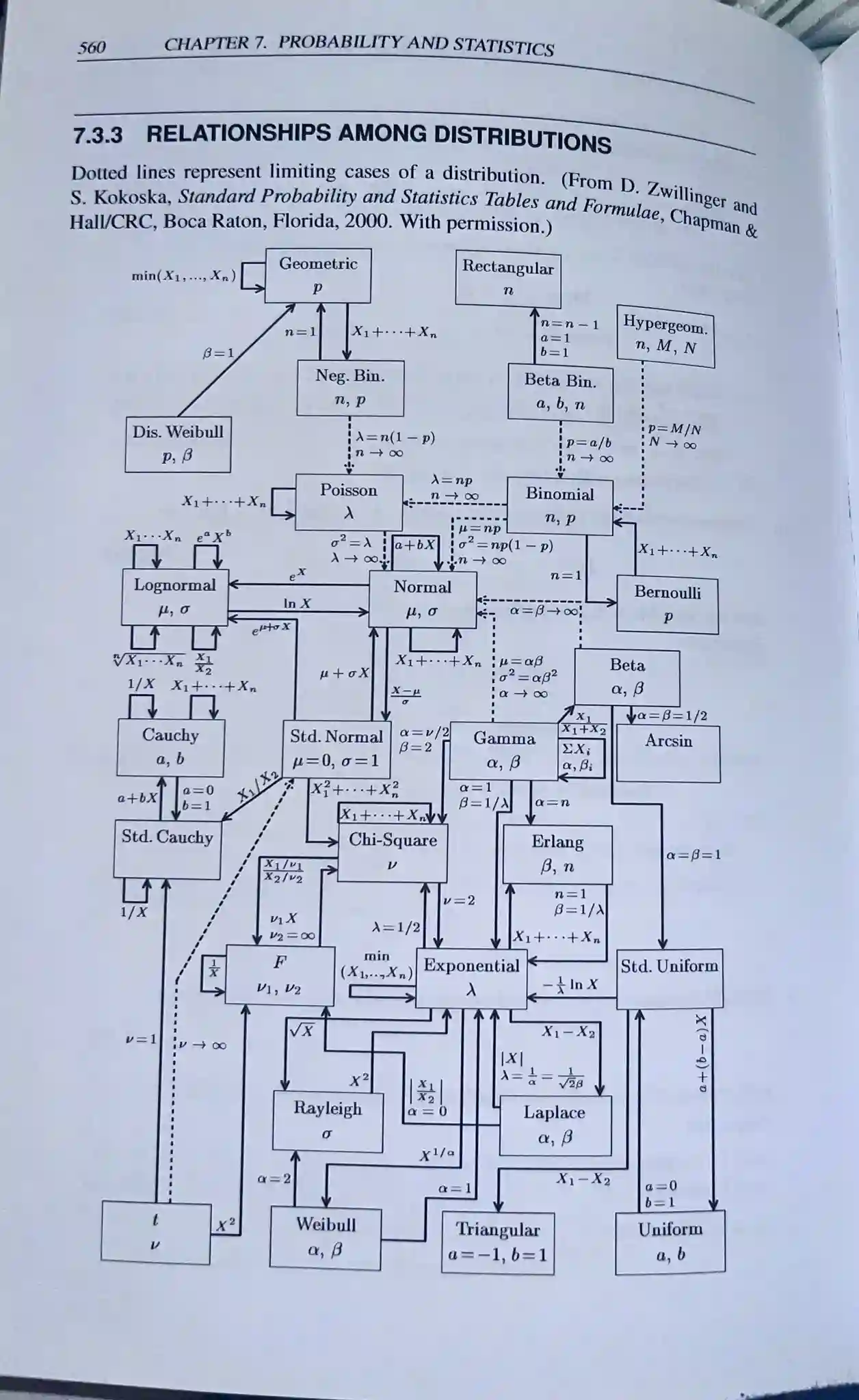
We used Gaussians to represent the uncertainty. Distributions are related: