Gaussian Mixture Models

This set takes inspiration from chapter 9.2 of (Bishop 2006). We assume that the reader already knows quite well what is a Gaussian Mixture Model and we will just restate the models here. We will discuss the problem of estimating the best possible parameters (so, this is a density estimation problem) when the data is generated by a mixture of Gaussians.

Remember that the standard multivariate Gaussian has this format:

$$\mathcal{N}(x\mid \mu ,\Sigma )=\frac{1}{\sqrt{2\pi }}\frac{1}{|\Sigma {|}^{1/2}}\exp \left(-\frac{1}{2}(x-\mu {)}^T{\Sigma }^{-1}(x-\mu )\right)$$

Problem statement

Given a set of data points $x_1,\dots ,x_n$ in ${\mathbb{R}}^d$ sampled by $k$ Gaussian each with responsibility ${\pi }_k$ the objective of this problem is to estimate the best ${\pi }_k$ for each Gaussian and the relative mean and covariance matrix. We will assume a latent model with a variable $z$ which represents which Gaussian has been chosen for a specific sample. We have this prior:

$$p(z)=\prod _{i=1}^k{\pi }_i^{z_i}$$

Because we know that $z$ is a $k$ dimensional vector that has a single digit indicating which Gaussian was chosen.

The Maximum Likelihood problem

The frequentist approach with Maximum likelihood is quite probable to give rise to particular edge-cases that make this method difficult to apply for this density estimation problem. Let's remember that in the case of Gaussian mixture models, our loss function is the following:

$$\underset{\pi ,\mu ,\Sigma }{\min }\log p(X\mid \pi ,\mu ,\Sigma )=\sum _{n=1}^N\log \left\{\sum _{i=1}^K{\pi }_i\mathcal{N}(x_n\mid {\mu }_k,{\Sigma }_k)\right\}$$

So our parameter space is the following

$$\Theta =\left\{{\pi }_k,{\mu }_k,{\Sigma }_k:k\le K\right\}$$

Let's see now a case where this function is not well behaved. Let's consider the covariance matrix to be ${\sigma }_i^{2}I$ and let's say we have sampled a single point that is exactly ${\mu }_i$ then we have that the contribution of this particular Gaussian to our loss function is

$$\mathcal{N}(x_n\mid x_n,{\mu }_i,{\sigma }_i)=\frac{1}{\sqrt{2\pi }{\sigma }_{{}_i}}$$

If we have a single point, and ${\sigma }_i\to 0$ which is reasonable because we have a single point on the mean, then this value explodes and makes the whole log-likelihood to go to infinity. This is a case we don't want to explore. There are some methods that try to solve this problem. But in this setting we don't want to explore this, and focus on the expectation maximization algorithm.

Ideas for the solution

Let's consider for instance the value $p(X,Z)$ this is a known value and it's equal to

$$\log p(X,Z)=\sum _{n=1}^N\log \left\{{\pi }_z\mathcal{N}(x_n\mid {\mu }_z,{\Sigma }_z)\right\}=\sum _{n=1}^N(\log {\pi }_z+\log \mathcal{N}(x_n\mid {\mu }_z,{\Sigma }_z))$$

That decomposition is quite nice. Having had this observation we can write our objective as

$$\log p(X)={\mathbb{E}}_{Z\sim q}\left[\log \frac{P(X,Z)}{P(Z\mid X)}\right]$$

Using product rule and using the expectation to get rid of the $Z$.

The interesting part comes when we multiply and divide by $q(Z)$ then we can decompose it further into two parts:

$$\log p(X)={\mathbb{E}}_{Z\sim q}\left[\log \frac{P(X,Z)}{q(Z\mid X)}\right]+{\mathbb{E}}_{Z\sim q}\left[\log \frac{q(Z\mid X)}{P(Z\mid X)}\right]=M(q,\theta )+E(q,\theta )$$

We note that $E$ is a Kullback-Leibler divergence so it's always positive, and we have $\log p(X)\ge M(q,\theta )$. The $M$ part is also known as the ELBO (see Variational Inference).

Another fundamental operation is that we can find the parameters of $q$ such that $E$ is null, because we know that if two distributions are the same then the divergence is null. We can compute this because we know the values of the posterior.

The expectation-maximization algorithm

Dempster et al., 1977; McLachlan and Krishnan, 1997 are useful references for this method.

Structure of the Algorithm

The algorithm in brief goes as follows:

1. Set an initial value ${\theta }^{(0)}$
2. for values $t=1,2,\dots$
   1. Set $q^{\ast }$ such that $E(q,{\theta }^{t-1})=0$, which is just minimizing this value.
   2. Set $\theta$ to the max of $M(q^{\ast },\theta )$. By adequately changing parameters for $p(X,Z)$ which is tractable.

From a more high level view:

1. Compute the posterior $\gamma$
2. Compute the best mean, variance and priors with the formula above and update them
3. Repeat until convergence.

It is guaranteed that the likelihood is increasing, but we might be stuck on local maxima and similar things.

Convergence of EM

This is just a bounded optimization problem, after which you use the convergence theorem in Successioni which asserts that the limit for bounded monotone sequences always exists and is Unique.

We know that $\log p(X)=M(q,\theta )+E(q,\theta )$, after the $E$ step, the corresponding Kullback-Leibler divergence is 0, so we have $\log p(X)=M(q^{\prime },\theta )$ where $q^{\prime }$ is the updated Variational estimator.

Then, if we set ${\theta }^{{}^{\prime }}=\arg {\max }_{\theta }\log p(X)=\arg {\max }_{\theta }M(q^{\prime },\theta )$, we have the following equations:

$$\log p_{{\theta }^{\prime }}(X)\ge M(q^{\prime },{\theta }^{\prime })\ge M(q^{\prime },\theta )=\log p_{\theta }(X)$$

Which is a increasing sequence. The upper bound is trivial, by axiomatic definition of $p$.

The importance of the class

If you assume to know the class for which the point $x$ is part of, then the problems becomes actually quite easy. This is the original problem that concerns k-means too! We don't know a priori which class has been used to generate the point $x$, so taking the expected value accounting for each possibility makes this usually quite hard.

This part corresponds to the E-step of the algorithm. In the case of Gaussian Mixture Models, this just corresponds setting $q(z)\sim p(z\mid x)$ Which is just:

$$q(z=i)=p(z\mid x_n)=\frac{p(x_n,z)}{p(x_n)}=\frac{{\pi }_i\mathcal{N}(x_n\mid {\mu }_i,{\Sigma }_i)}{{\sum }_j{\pi }_j\mathcal{N}(x_n\mid {\mu }_j,{\Sigma }_j)}=\gamma (z_{ni})$$

The Loss Function

It is possible to define a loss function with respect to the parameters $\pi ,\Sigma ,\mu$ after the variational posterior has been fitted in the $E$ step.

We denote

$$\gamma (z_{nk})=p(z_j\mid x_n)=\frac{p(x_n\mid z_j)p(z_j)}{{\sum }_{i}p(x_n\mid z_i)p(z_i)}=\frac{{\pi }_j\mathcal{N}(x_n\mid {\mu }_j,{\Sigma }_j)}{{\sum }_i{\pi }_i\mathcal{N}(x_n\mid {\mu }_i,{\Sigma }_i)}$$

Then we can write the loss function as

$$\begin{array}{r}\mathcal{L}(\pi ,\Sigma ,\mu )=\sum _{n=1}^N\sum _{k=1}^K\gamma (z_{nk})(\log |{\Sigma }_k|+\frac{1}{2}(x_n-{\mu }_k{)}^T{\Sigma }_k^{-1}(x_n-{\mu }_k)-\log {\pi }_k)\end{array}$$

Then you can derive this loss to get the best mean, Sigma and $\pi$. This follows (Murphy 2012), but I am not sure I modified it correctly.

Deriving the expected mean

Then we continue with the maximization step, which is finding the best variables under this new variational family.

First we want to do some multivariable analysis in order to derive some conditions of the minima, for this reason we take the derivative with respect to ${\mu }_k$ of the loss equation, and we derive that

$$\begin{array}{rl}\frac{\partial \log p(x)}{\partial {\mu }_k}& =\sum _{n=1}^N\gamma (z_{nk})\frac{\partial \log p(x_n,z_k)}{\partial {\mu }_k}\\ & =\sum _{n=1}^N\frac{{\pi }_k\mathcal{N}(x_n\mid {\mu }_k,{\Sigma }_k)}{{\sum }_j{\pi }_j\mathcal{N}(x_n\mid {\mu }_j,{\Sigma }_j)}\cdot \left(-\frac{1}{2}\right)\frac{\partial (x_n-{\mu }_k{)}^T{\Sigma }_k^{-1}(x_n-{\mu }_k)}{\partial {\mu }_k}\\ & ⟹-\sum _{n=1}^N\frac{{\pi }_k\mathcal{N}(x_n\mid {\mu }_k,{\Sigma }_k)}{{\sum }_j{\pi }_j\mathcal{N}(x_n\mid {\mu }_j,{\Sigma }_j)}{\Sigma }_k^{-1}(x_n-{\mu }_k)=0\\ & ⟹-\sum _{n=1}^N\gamma (z_{nk}){\Sigma }_k^{-1}(x_n-{\mu }_k)=0\\ & ⟹\sum _{n=1}^N\gamma (z_{nk})(x_n-{\mu }_k)=0\\ & ⟹{\mu }_k=\frac{1}{N_k}\sum _{n=1}^N\gamma (z_{nk})x_n\end{array}$$

Where $N_k={\sum }_{n=1}^N\gamma (z_{nk})$

we can interpret $N_k$ to be the number of points generated by the Gaussian $k$, and the internal part is just the weighted average of the points generated by $k$! This gives an easy interpretation of the mean of the expectation part of this algorithm.

Deriving the expected deviation

This one is harder, and I still have not understood how exactly this matrix derivative is done, but the end results is very similar to the above, we have

$${\Sigma }_k=\frac{1}{N_k}\sum _{n=1}^N\gamma (z_{nk})(x_n-{\mu }_k)(x_n-{\mu }_k{)}^T$$

Selecting the number of Clusters

You can check this in chapter 25.2 There is a problem at the beginning, even before you can apply the EM algorithm to estimate the probability, we need to choose the hyperparameter $k$ for the number of the classes that we are assuming to exist. We need a way to find a solution to find $k$ that could be more principled than just searching over the possible $k$ in a bruteforce manner.

With the stick breaking idea, we assume to have and infinite number of clusters. Then we will have some realizations of the clusters. We have the result that with $N\to \infty$ we will have a realization of every cluster. Having a realization means we have one member of $x$ that is part of this class.

We discover how to select this with the following section, where we delve into Dirichlet processes.

K-Means

The problem

Let's say we have a set of $d$ dimensional points $\mathcal{X}=\left\{x_1,\dots ,x_n\right\}$ We would like to learn a function

$$c:{\mathbb{R}}^d\to \left\{1,\dots ,k\right\}$$

That assigns each point some unique label.

We consider the prototype which is a representative of one class. In classical k-means we would like to minimize the the squared distance (or other distance function) for each example of the row. We can write:

$$R(c,\mathcal{Y})=\sum _{i=1}^N\Vert x_i-{\mu }_{c(x)}{\Vert }^2$$

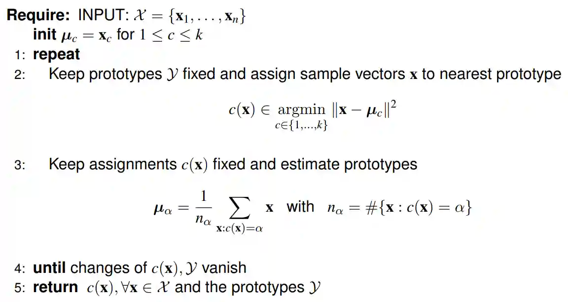
The Algorithm

References

[1] Bishop “Pattern Recognition and Machine Learning” Springer 2006

[2] Murphy “Machine Learning: A Probabilistic Perspective” 2012