There is a big difference between the empirical score and the expected score; in the beginning, we had said something about this in Introduction to Advanced Machine Learning. We will develop more methods to better comprehend this fundamental principles.

How can we estimate the expected risk of a particular estimator or algorithm? We can use the cross-validation method. This method is used to estimate the expected risk of a model, and it is a fundamental method in machine learning.

Validation methods

Cross-Validation

Cross validation is one of the oldest and most popular methods to validate our model parameters. The following slide summarizes the main idea of the cross-validation method.

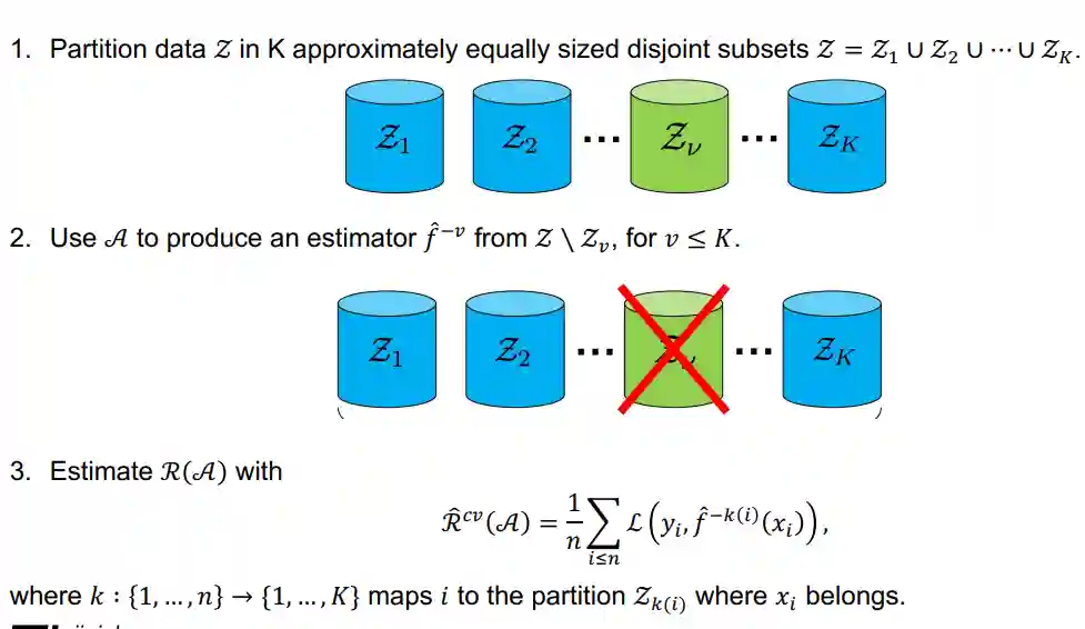
With this method we divide our dataset into $S$ buckets and use $S-1$ of those buckets to train and the rest to validate. If $S=N$ where $N$ is the size of the dataset this is usually called leave-one-out cross-validation. As with this method one needs to have $S-1$ training, this method is usually considered to be computationally expensive for the algorithms that need a lot of time to train.

Bootstrap

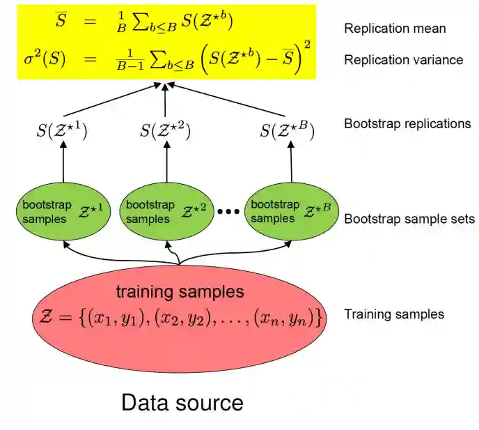
The bootstrap method is a resampling method that can be used to estimate the distribution of a statistic. The idea is to resample from the dataset with replacement and then calculate the statistic of interest. (Has the advantage of using the whole dataset instead of part of it, as Cross validation does) This process is repeated many times to estimate the distribution of the statistic. The bootstrap method is useful when the distribution of the statistic is unknown or when the sample size is small.

TODO: probability of one sample appearing in the bootsrap samples.

Each sample in bootstrap has a probability of appearing of $1-(1-\frac{1}{N}{)}^N\approx 1-e^{-1}\approx 0.632$. Taking this into account, we would need to rethink the computation of the risk splitting it into two cases: Risk = probability that sample is in the task $\times$ risk in this case + probability of not being in the sample $\times$ risk in this case. This can be rewritten as:

$$\text{Risk}=0.632\times {\text{Risk}}_{included}+0.368\times {\text{Risk}}_{excluded}$$

We can write then as:

$${\text{Risk}}_{included}=\frac{1}{N}\frac{1}{B}\sum _{b=1}^B\sum _{i=1}^{N}L({\theta }_b,x_i,y_i)$$

And

$${\text{Risk}}_{excluded}=\frac{1}{B}\sum _{b=1}^B\frac{1}{C^{-b}}\sum _{i\in C^{-b}}L({\theta }_b,x_i,y_i)$$

Hypothesis Testing

Hypothesis testing is like a legal trial. We assume someone is innocent unless the evidence strongly suggests that he is guilty. In (Wasserman 2004).

This seems to be a good resource for p-values.

P-values

We use p-values when we have a clear definition of the kinds of hypothesis that we are going to test. This value is useful if we want to compare two hypothesis: one that is the default safe assumption, and the other that is the surprising possible discovery. Usually we partition the parameter space $\Theta$ in two disjoint sets ${\Theta }_0$ and ${\Theta }_1$, where ${\Theta }_0\cap {\Theta }_1=\varnothing$ and ${\Theta }_0\cup {\Theta }_1=\Theta$. Then we have the null hypothesis $H_0$ and the alternative hypothesis $H_1$. We want to find a rejection region $R$ such that if the observed data falls in $R$ we reject the null hypothesis, otherwise we accept it.

Most likely the rejection region has the form

$$R_c=\left\{x\mid T(x)\ge c\right\}$$

Where $c$ is called the critical value and $T$ is the test statistic.

After we have defined those, we can define the p-value as

$$\text{p-value}=\inf \left\{\alpha :T(X^n)\in R_{\alpha }\right\}$$

where $R_{\alpha }$ is the rejection region of size $\alpha$. So the P-value tells us how likely are we to accept $H_0$, if it's small we are likely to reject it, if it's large we are likely to accept it. In practice, we often set the $\alpha$ value to be 0.05 as one does not have access to the real distribution of the data. So the p-value just tells us the probability of the null hypothesis to be true. Murphy highlights some questions regarding the validity of that statistics in section 6.6.2 of (Murphy 2012).

Types of error

• Type I error: Rejecting the null hypothesis when it is true.
• Type II error: Accepting the null hypothesis when it is false.

Type I error is usually much more serious than Type II error. It could lead to unintended actions that attempt to leverage on the false information, thus bringing demise. If we want are obliged to choose between one of those errors, one would prefer the Type II error. This is why we only accept the alternative hypothesis when there is strong evidence for it.

Risk of the least risky critical value that would lead to the rejection of the null hypothesis.

$$\text{p-value}=P(\text{observed data}|\text{null hypothesis})$$

Size and Power function

Given a rejection region $R$ we define the power function to be

$$\beta (\theta )={\mathbb{P}}_{\theta }(X\in R)$$

So, the power function is the probability of rejection and is more related to Type II errors.

We want our default hypothesis to be the safest as possible, so usually we consider his size $\alpha$ to be the one that has the greatest value:

$$\alpha =\underset{\theta \in {\Theta }_0}{\sup }\beta (\theta )$$

We say that a test has significance level $\alpha$ if its size is less or equal to $\alpha$. Usually the value that is picked is 0.05, but this is just tradition, the value is completely arbitrary.

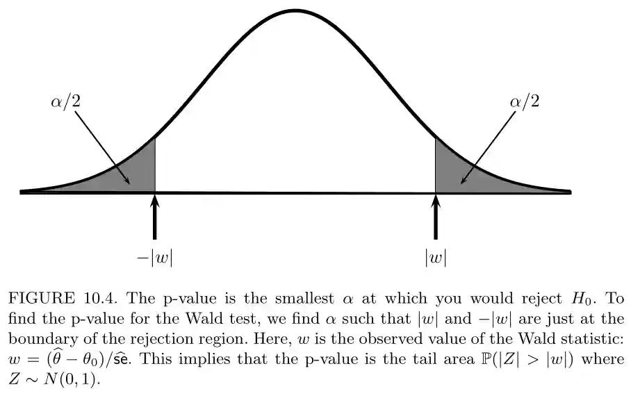
Wald Test

The wald test is defined as

$$W=\frac{\hat{\theta }-{\theta }_0}{\text{se}}\sim N(0,1)$$

Given a size $\alpha$ we reject if $|W|>z_{\alpha /2}$ where $z_{\alpha /2}$ is the $\alpha /2$ quantile of the standard normal distribution.

With this test the p-value is defined as

$$\text{p-value}=2\min \left(P(W<w),P(W>w)\right)$$

References

[1] Wasserman “All of Statistics: A Concise Course in Statistical Inference” Springer Science & Business Media 2004

[2] Murphy “Machine Learning: A Probabilistic Perspective” 2012