This set of note is still in TODO
Dependency Grammar has been much bigger in Europe compared to USA, where Chomsky’s grammars ruled. One of the main developers of this theory is Lucien Tesnière (1959):
“The sentence is an organized whole, the constituent elements of which are words. Every word that belongs to a sentence ceases by itself to be isolated as in the dictionary. Between the word and its neighbors, the mind perceives connections, the totality of which forms the structure of the sentence. The structural connections establish dependency relations between the words. Each connection in principle unites a superior term and an inferior term. The superior term receives the name governor (head). The inferior term receives the name subordinate (dependent).” ~Lucien Tesnière
This grammars defines binary relations between words. These relations are labelled. Dependency parsing is just having a tree representation of these relations. We can view dependency parsing as another way of understanding syntax in language.
Dependency Trees
Definitions
Let’s say all words in a sentences are nodes of a graph, plus a root node. A dependency tree is a directed spanning tree in the graph
- All non-root nodes have exactly one incoming edge
- No cycles
- Only 1 outgoing edge from the root
Types of Dependency Trees
We have two main kinds of trees
- Non-projective dependency trees: when they have some overlapping arcs, then it’s a non-projective dependency tree
- Projective dependency trees. they do not have overlapping arcs.
From Parse Trees to Dependency Trees
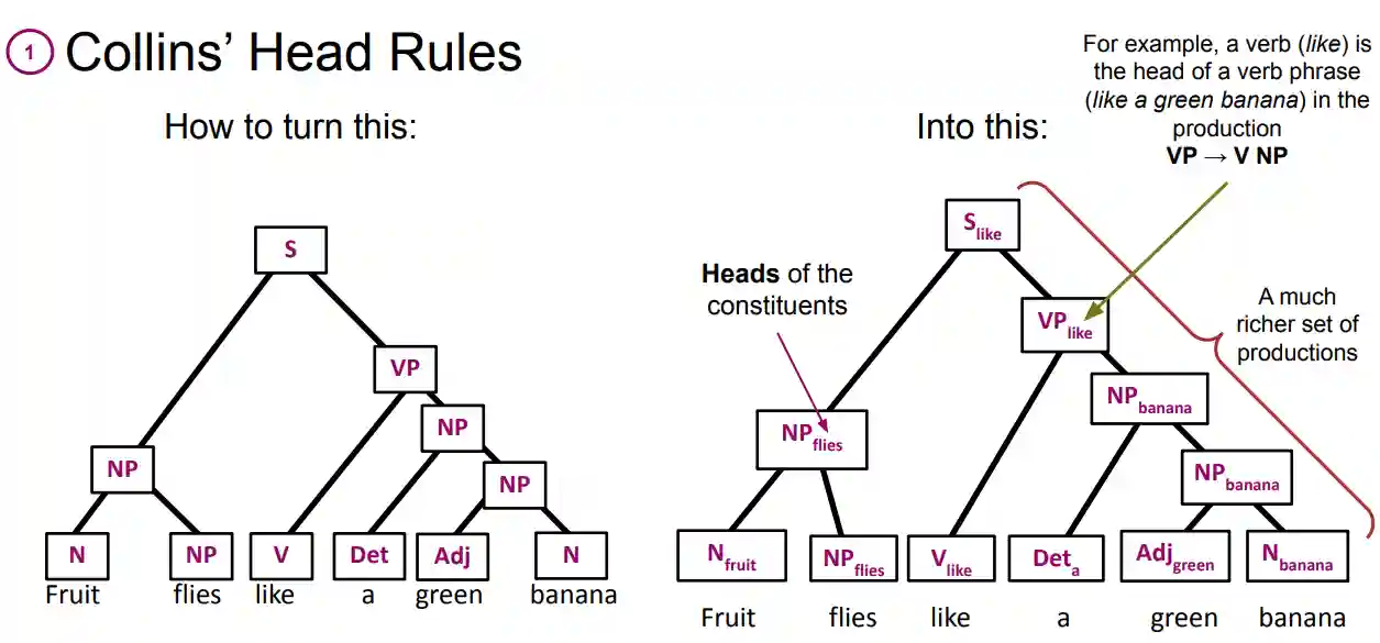
We covered parse trees in Probabilistic Parsing. There is a way to convert parse trees into dependency trees in a quick manner: Collin’s head rules
Collin’s head rules
See here. Usually when we have a parse tree, only one relation is linguistically plasible. Collin’s head rules just describe which one is plausible. For example, if we have adjective and noun, usually the noun is the head of the noun phrase.
 (Image from Course Slides, NLP ETH2024)
On the left we have a standard constituency tree, on the right, we have every non terminal labelled using Collin's head rules.
Constituency trees are Projective Dependency Trees
The title of this section quickly follows from the fact that syntactic constituents are contiguous, which implies we won’t have any crossings (somehow, I did not clearly understood this). So, if we have a projective dependency tree, we can easily build a probabilistic model for it following the machinery built in the previous chapter, in Probabilistic Parsing (CKY and similar dynamic programming based algorithms). Next, we will consider how we can build models for non-projective dependency trees.
Deconding Dependency Trees
We would like to find the most probable dependency tree among all the possible graphs we could have. This is a daunting task because the possible tree we could have is exponential, in the order of $\mathcal{O}(N^{N})$ where $N$ is the length of our sentence.
Kirchhoff’s Matrix-Tree Theorem
In this section we explore methods to compute the probability distribution over non-projective dependency trees.
Counting spanning trees
Given a Degree Matrix $D$ and the adjacency matrix $A$, we build the Laplacian Matrix $L = D - A$. We can compute the number of spanning trees of a graph by computing the determinant of the Laplacian Matrix. Remember that the determinant is computable in $\mathcal{O}(n^{3})$ time, so we can find the count in this amount of time.
Extending to root nodes
This is a contribution from Koo 2007. We modify the Laplacian Matrix to include the root node. TODO. The weird thing is that we just need to substitute the first row with the scores of the roots. And it will work. In the paper there are the details of the equivalency. A good thing would be spending one hour actually undersanding why the determinant of the following matrix does the job
$$ L_{ij} = \begin{cases} \rho_{j} & \text{if } i = 1 \
- D_{ij} & \text{if } i \neq j \ \sum_{i’ = 1, i’ \neq j}^{N} D_{i’j} & \text{if } i = j \end{cases} $$ There $D_{ij}$ is the score of the edge between $i$ and $j$, and $\rho_{j}$ is the score of the edge between the root and $j$.
Chu-Liu-Edmonds Algorithm
See this resource, it is well made and has also an implementation in python with some visualizations.