The DP (Dirichlet Processes) is part of family of models called non-parametric models. Non parametric models concern learning models with potentially infinite number of parameters. One of the classical application is unsupervised techniques like clustering. Intuitively, clustering concerns in finding compact subsets of data, i.e. finding groups of points in the space that are particularly close by some measure.
The Dirichlet Process
See Beta and Dirichlet Distributions for the definition and intuition of these two distributions. One quite important thing that Dirichlet allows to do is the ability of assigning an ever growing number of clusters to data. This models are thus quite flexible to change and growth.
Definition of the process
A Dirichlet Process is a distribution over probability measures . It is defined as:
Where given a partition of our sample space into a countable number of disjoint sets we have that:
So they are jointly distributed as a Dirichlet distribution. And is called the base measure and is called the concentration parameter.
The base measure represents our prior belief about the distribution of the data. is called concentration parameter: is small, the resulting distributions tend to concentrate on fewer clusters, effectively encouraging sparsity. Conversely, a larger allows for a richer, more diverse set of clusters.
Choosing number of Clusters
Dirichlet processes are related to finding the best number of clusters (See Clustering). It is a non-parametric way (meaning it can grow with the data) to find that number.
Stick Breaking
We have dome something similar to in Gaussian Processes: the difference is sequential sampling compared to sampling all of the points at once using the difficult multivariate distribution.
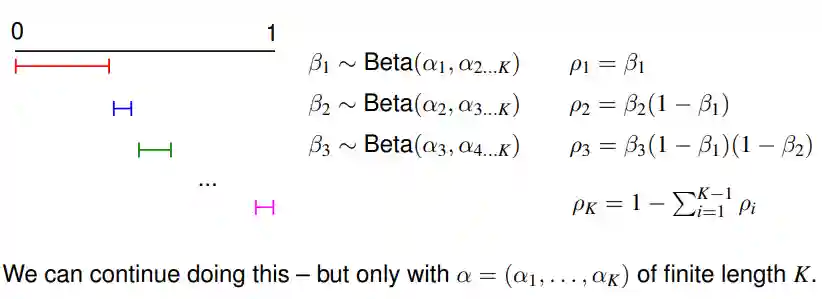
We would like to sample . So now we just sample the first and then sample the second conditioned on the first observation (So we have a beta distribution now) and so on, until we finish the possible clusters.
Image from the slides.
Griffiths-Engen-McCloskey distribution
This distribution is just a generalization of the stick breaking process. We write which means breaking according the distribution . if alpha is smaller then the stick is longer. So we can interpret the parameter as some sort of variable of the remaining stick length.
Using the above image, we can define the stick breaking patterns using constant values , which correspond to GEM distribution, a dirichlet process with concentration measure and base measure .
De Finetti's theorem
We define an infinite sequence of random exchangeable when it satisfies
with a permutation of the set .
Given a sequence of infinitely exchangeable sequence of random variables, then there exists a random variable such that :
Which means we can decompose the infinite exchangeable sequence into independent conditional random variables.
In the context of CRP and Urns, this property allows us to count the probability of ending into a specific number of clusters, each with some number of elements.
Classical Combinatorial problems
The Chinese Restaurant Process
We have some customers (observations) assigned to some clusters . Then we have the Matthew effect: more people in a table makes it more probable to seat there. Or some probability to create a new table .
So the probability of customer joining table and is the set of tables.
Given this modelling, then it's easy to compute the probability of a given table assignment, which is:
We can do this because it is order and labeling-independent. With this model, we can show that the expected number of table is in the order of In economy, this effect is called rich get richer because more popular cluster are able to attract more points into it.
Rate of increase of the number of tables
This number is important to track to get a sense of how the number of clusters is growing. Let's call a random variable that returns the number of tables after customers have been seated. Then the expected increase at each step is equal to the probability of creating a new table (if it's easier for you reader, you can also create an indicator variable that tells you if it has increased at step , call it ):
Then the expected number of tables after customers is:
This is a simple consequence of the bound of the harmonic series. See Serie.
Pólya Urns
We have urns with colored balls that can be drawn at random. If a ball is drawn it is doubled and put both back into the Urn. We can prove that this is equivalent to the Chinese Restaurant Process, given a finite number of clusters (colors). The important part is that this is exchangeable.
Hoppe Urn
This is a variation of the Pólya's urn. Here we have a special ball that when it's picked it is put back into the urn but also a new color is put back! Then this model is exactly the same as the Chinese Restaurant Process. It should be a nice exercise to prove this.
We can interpret the random variable in De Finetti's theorem as a single sample from the an underlying Dirichlet Process. After we have sampled this (which is a prior, it is like we are sampling hyperparameters), then we use CRP to assign the points to the clusters.
The DP Mixture Model
The model
We have the probability of the clusters
- and alpha is chosen appropriately with some validation.
- are the centers of the clusters.
- We draw some assignments to the clusters with a categorical distribution based on . We call these .
- We points , based on the above cluster parameters.
The easy way to remember this model is with a graphical model:
Fitting a learner
EM (see Clustering) are difficult to use for non-parametric models. We will use Gibbs Sampling introduced in Monte Carlo Methods.
With Gibbs we need to be able to compute the posterior . It's easy to see (also by using the independence assumptions of the graphical model) that this is proportional to:
And then we have the probabilities in the image.
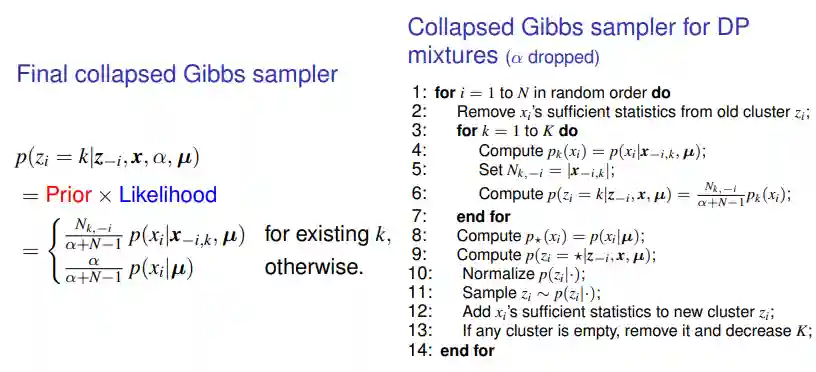
Code Example just run it on a Notebook. I noticed that if we initialize the code with all classes assigned to a single cluster, the model seems to fail to learn that there are other classes, this is probably because the rich get richer effect is not enough to explore the space of the clusters. If we initialize the code with a random assignment on the maximum number of clusters, then it doesn't seem to be able to eliminate clusters correctly. It is quite probable that we would need to tune for the value, but it is probably quite time consuming to find one.
A More Detailed Walk-Through
Let’s outline the steps more algorithmically:
-
Initialization:
- Initialize the cluster assignments arbitrarily (for example, each data point in its own cluster or by some heuristic).
- For each unique cluster, initialize the parameter by drawing from or by using an initial estimate from the assigned data.
-
Gibbs Sampling Loop: For each iteration, and for each data point : a. Remove from its current cluster:
Adjust the counts for the cluster that belonged to. If this removal makes the cluster empty, remove the cluster altogether. b. Compute assignment probabilities:- For each existing cluster :
- For a new cluster: is the marginal likelihood for under the base measure. c. Sample a new assignment for from the discrete distribution defined by . d. If a new cluster is chosen:
- Draw a new parameter from the posterior given (or directly from if you wish to assign it prior to any data update).
e. Update Cluster Parameters:
For each cluster , sample
-
Convergence and Inference: After a sufficient number of iterations, the samples of and represent draws from the posterior distribution of the DP mixture model. You can then estimate cluster structures, predictive densities, or other quantities of interest.
Drawbacks of Dirichlet
We provide here a summary of the main drawbacks of the Dirichlet Process:
| Category | Drawback |
|---|---|
| Growth Assumptions | Logarithmic growth may not fit real-world data |
| Cluster Size Bias | Overemphasis on large clusters; poor handling of outliers |
| Hyperparameter Sensitivity | Choice of and (Base Measure) affects clustering |
| Inference Complexity | MCMC/Variational methods are computationally expensive |
| Exchangeability Assumption | Fails for temporally or spatially structured data |
| Expressiveness | Limited ability to handle complex or hierarchical data relationships |
| Scalability | Standard DP methods struggle with large datasets |
| Task Restriction | Primarily a clustering tool, requiring extensions for other tasks |
We observe that the main points are the exchangeability assumption, the growth assumptions (in real life some clusters may grow linearly or exponentially), and the scalability.