Monte Carlo Methods

DI Law of Large Numbers e Central limit theorem ne parliamo in Central Limit Theorem and Law of Large Numbers. Usually these methods are useful when you need to calculate following something similar to Bayes rule, but don't know how to calculate the denominator, often infeasible integral. We estimate this value without explicitly calculating that.

Interested in $\mathbb{P}(x)=\frac{1}{z}{\mathbb{P}}^{\ast }(x)=\frac{1}{Z}{e}^{-E(x)}$ Can evaluate E(x) at any x.

• Problem 1 Make samples x(r) ~ 2 P
• Problem 2 Estimate expectations $\Phi ={\sum }_x\varphi (x)\mathbb{P}(x)$) What we're not trying to do:
• We're not trying to find the most probable state.
• We're not trying to visit all typical states.

Law of large numbers

Data una sequenza di variabili aleatorie, $X_1,X_2,\dots ,X_n\dots$, tali che siano i.i.d tali per cui $E(X_1)=E(X_2)=\cdots =E(X_n)=\cdots =\mu$ tale che sia finito. Consideriamo

$$S_n=\sum _{i=1}^n{x}_i,:,{\bar{x}}_n=\frac{S_n}{n}$$

Allora questo teorema afferma che:

$${\bar{x}}_n\to \mu$$

Ossia il limite converge sul valore atteso di tutte le variabili aleatorie.

Inoltre se abbiamo che la varianza di tutte le variabili aleatorie, abbiamo che

$$var({\hat{x}}_n)=\frac{{\sigma }^2}{n}\to 0$$

Strong Law of large Numbers

$$\mathbb{P}(\underset{n\to \infty }{\lim }{\bar{x}}_n=\mu )=1$$

Ci permette di prendere la sample average per quei valori di mezzo. E posso fare la stima della nostra funzione di interesse $h$ tenendo conto:

$${\bar{h}}_n=\sum _{i=1}^n\frac{h(x_i)}{n}$$

E questo converge $O(\sqrt{n})$ per la legge dopo.

Central limit theorem

Data una sequenza di variabili aleatorie, $X_1,X_2,\dots ,X_n\dots$, tali che siano i.i.d tali per cui $E(X_1)=E(X_2)=\cdots =E(X_n)=\cdots =\mu$ tale che sia finito, e con varianza tutti uguali $={\sigma }^2$ finito.

Abbiamo come risultato che

$$\sqrt{n}({\hat{x}}_n-\mu )\to N(0,{\sigma }^2)$$

La prima parte è una variabile aleatoria e converge a quel valore. (questo permette di utilizzare la gaussiana quando $n$ è grande abbastanza).

Monte carlo integration

Abbiamo che:

$${\int }_{X}h(x)\cdot f(x)dx=E_f[h(x)]=\mu$$

Questo è tutto il significato dell'integrazione di monte carlo (molte variabili aleatorie per stimare il valore di qualcosa). E questo vale sempre, anche se $f$ non è una funzione di densità, basta che sia positiva (basta riscalare).

Il motivo per cui funziona è per LLN, perché abbiamo che convergerà su $\mu$ in lungo termine, basta considerare molte variabili aleatorie consecutive.

Cose interessanti:

1. Posso stimare il valore atteso grazie a LLN
2. Posso stimare la varianza grazie ad essa
3. Posso stimare variabili condizionali.

Importance sampling

1. Deve soddisfare la cosa del supporto (contiene supporto sia di h che di f)
2. Deve avere varianza finita per i pesi che sono trovati. (ci sono metodi per stimare poi il $g$).
   1. la frazione $\frac{f}{g}$ deve essere limitata e la varianza di $h$ rispetto alla densità $f$ deve essere finita.

Bound on samples

TODO: this should be interesting and important and should use Hoeffding's inequality.

Markov Chain Monte Carlo

L'idea principale di Markov Chain Monte carlo è di costruire una catena di Markov tale che si possa utilizzare per generare dalla distribuzione difficilmente trattabile. Uno dei metodi principali per fare ciò è utilizzare tecniche si sampling.

Metropolis Hastings

The Sampling Algorithm

We observe that this sampling algorithm takes idea from Markov Chains balanced equation's property of stationary distributions and the Accept Reject algorithm for sampling some distributions. Also in this case, we don't care about the normalization constant for $p$, the distribution that we would like to sample from. We choose the that acceptance probability as it allows us to satisfy the balance equation and thus, the stationary property of the constructed Chain.

With Metropolis-Hasting we need to

1. Be able to calculate the density for the target distribution
2. Be able to sample easily from the $q$ distribution. Then it has some links with Random Walks inside the space we want to sample.

With Metropolis Hastings we accept with probability

$$\alpha =\min \left(1,\frac{p(x^{\prime })q(x\mid x^{\prime })}{p(x)q(x^{\prime }\mid x)}\right)$$

Where $x$ is the current state and $x^{\prime }$ is the proposed state.

Stationary Distribution

We can prove that with that acceptance rate, the probability of transitioning in a given state satisfies the balance equation for the stationary distribution, which implies we can have a well behaved Markov Chain, and continue to sample from this.

We see that the probability of transitioning from $x$ to $x^{\prime }$ is the same as transitioning from $x^{\prime }$ to $x$.

$$p(x)q(x^{\prime }\mid x)\alpha =p(x^{\prime })q(x\mid x^{\prime })\alpha$$

To prove this, just consider the two possible cases for the min function.

Con distribuzioni Gaussiane

Il caso continuo con distribuzione Gaussiane potrebbe essere di particolare interesse perché semplifica l'analisi del calcolo del coefficiente $\alpha$: dato che le Gaussians sono simmetriche, abbiamo che il valore di

$$\frac{r(x^{\prime }\mid x)}{r(x\mid x^{\prime })}=\frac{\mathcal{N}(x^{\prime };x,\tau I)}{\mathcal{N}(x;x^{\prime },\tau I)}=1$$

Quindi il coefficiente $\alpha$ si può scrivere anche solo come le distribuzioni $\frac{q(x)}{q(x^{\prime })}$ che se si assume una distribuzione di Gibbs, si può intendere come un $\exp (f(x)-f(x^{\prime }))$, che è di facile interpretazione. Quindi possiamo fare sampling solamente considerando il rapporto fra le due distribuzioni.

Variations and Improvements

Metropolis-Hastings' sample efficiency could be improved by adding information about the gradient of the distribution. This is the idea behind the Langevin algorithm.

Metropolis Adjusted Langevin Algorithm

The Metropolis-Adjusted Langevin Algorithm (MALA) modifies the Metropolis-Hastings method by incorporating gradient information of the target distribution to guide proposals, fixing the mean with a gradient descent step. Now the mean is $x-\tau \nabla f(x)$ instead of just $x$. The proposal function is still a Gaussian. This allows us to accept always, which motivates why it is more efficient compared to the Metropolis Hasting algorithm. Now the proposal distribution is the following

$$r(x^{\prime }\mid x)=\mathcal{N}(x^{\prime };x+\tau \nabla f(x),2\tau I)\propto \exp \left(-\frac{1}{2}{\Vert \frac{x^{\prime }-x-\tau \nabla \log p(x)}{G}\Vert }^2\right),$$

§ It is possible to show that for log-concave distributions (e.g., Bayesian log. Regression), MALA efficiently converges to the stationary distribution (mixing time is polynomial in the dimension)

Somehow, one can prove that if $\tau \to 0$ then the Metropolis Hastings tends to always accept the proposal, which is why it is more efficient. The version of Metropolis Hastings that always accepts is called Unadjusted Langevin Algorithm.

If we model the energy function as:

$$p(\theta \mid x_{1:n},y_{1:n})=\frac{1}{Z}\exp (\log p(\theta )+\sum _{i=1}^n\log p(y_i\mid x_i,\theta ))$$

Similarly to a Log Linear Models in language processing, then the update function is the following:

$${\theta }_{t+1}={\theta }_t+\tau {\nabla }_{\theta }\log p(\theta )+\tau \sum _{i=1}^n{\nabla }_{\theta }\log p(y_i\mid x_i,\theta )+\epsilon$$

Where $\epsilon \sim \mathcal{N}(0,2\tau I)$

The drawback of this method is that computing the energy for the whole dataset is expensive for large datasets. This is why sometimes we use a stochastic version of this algorithm. Which drives to the stochastic gradient Langevin dynamics.

Stochastic Gradient Langevin Dynamics

The double value for the Noise signal is justifiable if you study diffusion processes. So if you want to know how the $2$ factor comes into play when analyzing the process take a look at those courses. One can also estimate the update of the gradient of the likelihood by having $m$ samples and then using that values for the update: So the algorithm for the update becomes:

1. Sample $m$ points and then update $\theta$ as follows:

$${\theta }_{t+1}={\theta }_t+\tau {\nabla }_{\theta }\log p(\theta )+\tau \frac{n}{m}\sum _{i=1}^m{\nabla }_{\theta }\log p(y_i\mid x_i,\theta )+\epsilon$$

Langevin Monte Carlo

TODO: this is just an Outlook, and it is left out from here.

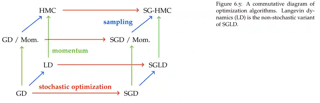
Landscape of sampling methods

we can broadly categorize optimization methods based on the use of

• Momentum
• Stochasticity
• Sampling Then we would have this cube.

Gibbs Sampling

These are probably not very important for the exam. We use a collapsed version of Gibbs Sampling for Dirichlet Processes.

The Idea

Gibbs sampling is a special case of Metropolis Hasting, in this case the proposal distribution $r$ is as follows:

$$r_i(x^{\prime }\mid x)=\{\begin{array}{ll}p(x_i^{\prime }\mid x_{-i}^{\prime })& \text{if }{x}^{\prime }\text{ differs from }x\text{ only in }i\\ 0& \text{else}\end{array}$$

We just focus on a single coordinate difference. Similar to the coordinate descent in some manner.

Proof of correctness

This sections proves that Gibbs Sampling indeed gives the original distribution. We will use a similar idea presented for #Metropolis Hastings.

One can observe the following:

$$\begin{array}{r}{\alpha }_i(x^{\prime }\mid x)=\min \left(1,\frac{p(x^{\prime })}{p(x)}\right)=1\end{array}$$

A simple code example

This code example shows how we can sample from a multivariate Gaussian using Gibbs sampling. Note that we just need to be able to compute marginals in order to sample this.

import numpy as np
import matplotlib.pyplot as plt

# Define parameters of the bivariate Gaussian
mu1, mu2 = 0, 0 # Means
sigma1, sigma2 = 1, 1 # Standard deviations
rho = 0.8 # Correlation coefficient

# Derived quantities
cov = rho * sigma1 * sigma2 # Covariance
Sigma = np.array([[sigma1**2, cov], [cov, sigma2**2]]) # Covariance matrix
Sigma_inv = np.linalg.inv(Sigma) # Precision matrix


# Conditional distributions
def sample_x1_given_x2(x2, mu1, mu2, sigma1, sigma2, rho):
	cond_mean = mu1 + rho * (sigma1 / sigma2) * (x2 - mu2)
	cond_var = (1 - rho**2) * sigma1**2
	return np.random.normal(cond_mean, np.sqrt(cond_var))

  
def sample_x2_given_x1(x1, mu1, mu2, sigma1, sigma2, rho):
	cond_mean = mu2 + rho * (sigma2 / sigma1) * (x1 - mu1)
	cond_var = (1 - rho**2) * sigma2**2
	return np.random.normal(cond_mean, np.sqrt(cond_var))

# Gibbs Sampling
def gibbs_sampling(num_samples, burn_in=100):
	samples = []
	x1, x2 = 0, 0 # Initial values
	for _ in range(num_samples + burn_in):
		x1 = sample_x1_given_x2(x2, mu1, mu2, sigma1, sigma2, rho)
		x2 = sample_x2_given_x1(x1, mu1, mu2, sigma1, sigma2, rho)
		samples.append((x1, x2))
	return np.array(samples[burn_in:]) # Discard burn-in samples

# Run Gibbs Sampling
num_samples = 5000
samples = gibbs_sampling(num_samples)
  

# Plot results
plt.figure(figsize=(8, 6))
plt.scatter(samples[:, 0], samples[:, 1], alpha=0.5, s=5, label="Samples")
plt.title("Gibbs Sampling: Bivariate Gaussian", fontsize=14)
plt.xlabel("$X_1$", fontsize=12)
plt.ylabel("$X_2$", fontsize=12)
plt.axhline(0, color='gray', linewidth=0.5)
plt.axvline(0, color='gray', linewidth=0.5)
plt.grid(alpha=0.3)
plt.legend()
plt.show()