In this note we will first talk about briefly some of the main differences of the three main approaches regarding statistics: the bayesian, the frequentist and the statistical learning methods and then present the concept of the estimator, compare how the approaches differ from method to method, we will explain maximum likelihood estimator and the Rao-Cramer Bound.
Short introduction to the statistical methods
Bayesian
With bayesian methods we often assume a prior on the parameters, often human picked, that allows to give a regularizer term over the possible distribution that we are trying to model. The prior is just an assumption on the distribution of the model and the likelihood , where are the features, and the model. After we have these two distributions defined, we can then use the famous Bayes rule to compute the posterior, and chose the best possible model given our dataset in this manner. This induces a distribution over possible that we can consider. Another characteristic is that the Bayes' rule is often infeasible to compute practically. So what we compute is
The quantity could be very complicated if our model is complicated.
Frequentist
Fisher founded this view of statistics. (Murphy 2012) has a nice Chapter (6) about this topic. Frequentist methods start by having assumptions on the space of the model parameters (this is the class), so we have a family of models , but now this assumption is not a belief on the data itself, instead, a restriction that you have to pose in order to limit your search space (the need arises from practical purposes, not from beliefs, we want the most general possible models). Another aspect of frequentism is conditioning only on the observed data, and not on any priors. This methods leads to certain paradoxes of this type of modeling. But then, instead of using the Bayes' rule, they just try to maximize the possibility that a certain has given rise to that data. In formulas we have:
We assume the data is i.i.d so we need to estimate this value:
This is how maximum likelihood estimators naturally arise with the frequentist approach. This is asymptotically true.
Usually with enough data and big models, frequentist's methods are preferred.
Statistical learning
The last possible interpretation, the statistical learning approach, I think is due to (Vapnik 2006)'s studies on Statistical learning theory, asserts that the best method is the one that minimizes the risk, meaning it should have the least error on the test split of our dataset. This risk is not accessible so we need to minimize the empirical risk So we try to chose the is this way:
So we choose an approximation for the risk which is
And then choose the best from his family of functions
Three problems in statistical learning
The goal of statistical learning is to find a function such that the error rate is minimized. We define the error rate to be just the cases where . Let's have so a simple model:
So we want to minimize the following value:
- We don't know anything about , we need to have some assumptions, the easiest is to define a hypothesis class.
- We don't know the starting distribution , we solve this by collecting training samples so that we have an estimate of the starting distribution. (This is the fundamental problem in machine learning, we have empirical distribution, never the true distribution!)
- The risk is not differentiable, we solve this by choosing a loss function such that this is differentiable. We can write the starting problem in the following way as a proxy for the expected value.
This image summarizes the whole pipeline
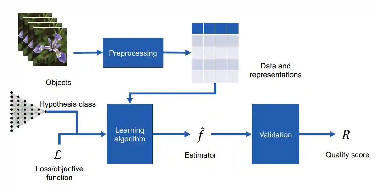
Let's have a simple example. Let's attempt to chose the hypothesis class for the iris setosa classification problem. We arbitrarily choose and to be
Then we can use Bayes rule to find and we can define then a simple loss, for example the classical binary cross entropy loss.
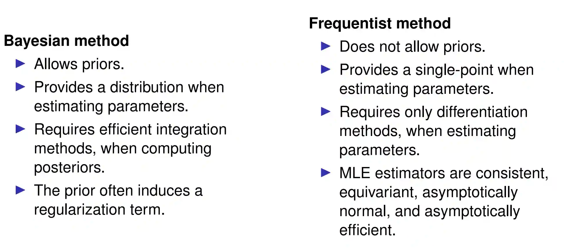
Bayesian and Frequentist head to head
Estimators
Estimators are functions or procedures that in this context of parametric models allow us to pin-point the correct parameters , in the case of the frequentist view, or give a distribution over possible s. Usually the generating function is called a density function parameterized by the so we have to define the class of models and likelihood first.
We will mainly focus in this setting with the Maximum likelihood estimator
The Maximum Likelihood Estimator
Given an assumption on the likelihood, we define the Maximum likelihood function to be
Definition of MLE
We define the Maximum Likelihood Estimator (MLE) to be simply the best maximum likelihood
Sometimes is useful to consider the log-likelihood because sums are usually easier to handle. We will indicate the log version with . Usually the loss is the likelihood of the data, this is why it's called Maximum Likelihood estimator.
Properties of the MLE
The important thing here is to be able to name the properties, not prove them. You can see a good presentation of these properties with (Wasserman 2004) chapter 9 (page 127 on wards). Three main properties concern us:
- Consistency: (meaning it will converge to the true parameter, if modelling assumptions are correct e.g. function family)
- In formula it means that a point estimator of a is consistent if it converges in probability which is:
- See [[Central Limit Theorem and Law of Large Numbers]] for definition of convergence in probability, the proof is not trivial and has many technicalities.
2. Asymptotic efficiency: For well-behaved estimators, the MLE has the smallest variance for large . - For example the median estimator satisfies , but the MLE doesn't have that factor. 3. Asymptotically normal: meaning the error will be Gaussian if we have too many samples. Which means that
- Informally, this theorem states that the distribution of the parameters $\theta$  that we find with MLE follows a normal distribution $\mathcal{N}(\theta_{*}, se)$. This theorem holds also for estimated standard errors. The interesting thing is that with this method we can build **asymptotic confidence intervals** for MLE, which can come quite handy in many occasions, and rival the bayesian approach for confidence intervals.
- The proof is quite hard, it is presented in the appendix of Chapter 9 of [[@wassermanAllStatisticsConcise2004]].
- Equivariance meaning: if is MLE of then for any given we have that is the MLE of . I don't know what is this useful for, but nice to know.
We will discuss these properties one by one. These properties are the reason why MLE is preferred over other estimators, such as means or medians.
We want to say that an estimator is efficient if it uses its information well, which means
Where is the fisher information. Every estimator is lower bounded by this. (this is the maximum efficiency) and it's very important.
Biases usually are good if it includes information that is correct with the data. (helps it learn faster, an example of why bias works is the Stein estimator, but I didn't understood exactly why). Simple cases and reasoning for first principles usually helps you build the intuition to attack more complex cases. This is something you would need to keep in mind.
MLE is overconfident
See Sur and Candes 2018
One can show that there are many examples where logistic regression (see Linear Regression methods) is quite biased. This is a problem especially with high dimensional data. There are some numerical instabilities with correlated features, especially when we are trying to invert something small (floating point imprecisions!)
You can see it quite easily: Remember that the ordinary least squares solution is , let's suppose we use Singular Value Decomposition and write then we have Inverting this we get and multiplying with the original one we get but the matrix is quite unstable, especially when you are inverting small numbers.
One nice thing about this decomposition is that the inference is just and that is a nice form.
Rao-Cramer Bound
Professor says this bound has same principle with the Heisenberg's uncertainty principle with the Cauchy-Schwarz inequality somehow. But I don't know about that. Rao-Cramer bound is a general bound on the variance of any unbiased estimator. This is the least possible error for unbiased estimator, which is a way to say that you know that you got the best for that class of functions.P
Let's consider a likelihood , for which is our parameter space, and some samples , using a particular . We want to know how precisely can we estimate the value given samples. So let's define an estimator and consider the expected deviation , which tells us how much can the estimated value vary compared to the ground truth. One nice thing is that this holds for every distribution.
Score function
We consider the value of a score to be (use the log because perhaps the could be large, and we try to see how much it varies when varying the parameters, we are interested in this value because you know, Massimi minimi multi-variabile, if it's 0 it should have some nice properties regarding maximum value of our likelihood).
Let's define the bias to be
Now let's consider the value of the expected score:
which is an interesting result.
Score estimator Covariance
Let's consider another value:
And the first part is surprisingly the bias of our estimator, so we want to see how much we can lower the bias value when we want to assess these kinds of problems.
We now consider the cross correlation between and
We now use Cauchy-Schwarz Inequality to observe that
We now expand the second term:
Which is just
Final Bound
Putting everything together we have that
If we have an unbiased estimator, which means that then we have that the expected difference of the models is always greater than the expected value of the double power of the score, also known as the fisher information in maths:
If instead we have a biased estimator, sometimes is advantageous because the numerator could actually be smaller.
Fisher information
If the information is high, it means the log likelihood changes fast. This is measure of information of how X changes with respect to .
Definition of Fisher information
Fisher information is defined as the variance of the score function. We discovered that the fisher information has something to do with the Rao-Cramer bound, let's briefly analyze that:
Where is the fisher information, the expected value of the squared score function.
We can also define the Fisher information as the Variance of the score function i.e. :
And simplifying, as we know that the mean of the score function is 0.
Fisher information could also be written as the derivative with respect of theta of the score function, if is twice differentiable. See wikipedia.
The Multi-variable case
Let's consider this
And assuming we have independent variables we can see with some tricks and reasoning about the mean that:
Which is a nice property of the fisher information
Fisher for Gaussian
The fisher information for the mean of the Gaussian is:
This means that the variance of the estimator is upper bounded by this value thanks to the Rao-Cramer bound:
Since the MLE estimate has indeed that variance, then we say it is efficient unbiased, it hits the lower bound of the variance.
Stein estimator
If we use this estimator we have that it is consistently better than the MLE, but we can't prove that this is the best ever possible. This has been known as stein's paradox for some time. See here. This video gives a nice intuition about Stein's estimator, you can visualize it as a biased estimator that concentrates variance by warping the space closer to the origin, so that all the candidate solutions are acqually closer to the true solution.
We have to assume we have a multivariate random variable with with the exact details are not important, but we want to say that MLE is not always the best, this is the surprising fact.
We then have that
References
[1] Murphy “Machine Learning: A Probabilistic Perspective” 2012
[2] Vapnik “Estimation of Dependences Based on Empirical Data” Springer 2006
[3] Wasserman “All of Statistics: A Concise Course in Statistical Inference” Springer Science & Business Media 2004