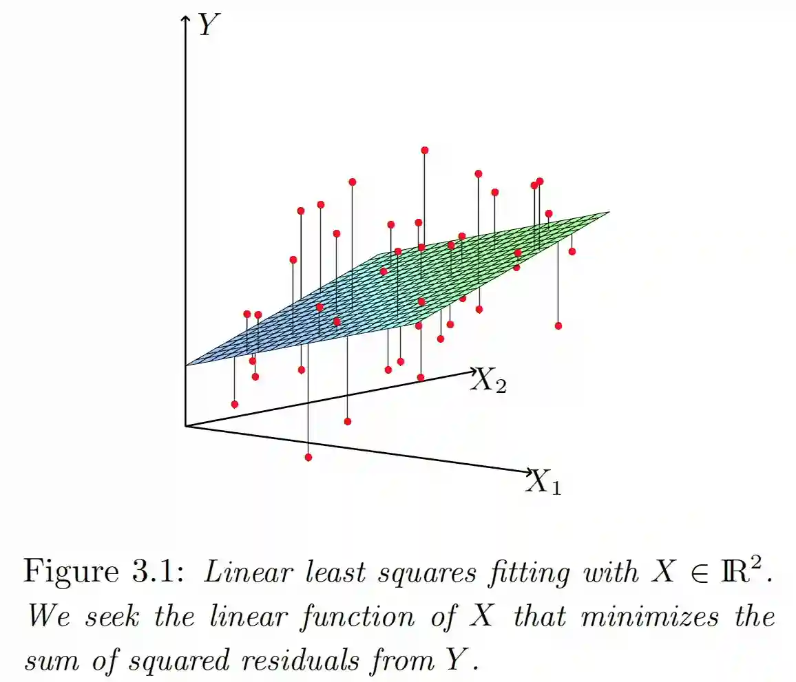
We will present some methods related to regression methods for data analysis. Some of the work here is from (Hastie et al. 2009). This note does not treat the bayesian case, you should see Bayesian Linear Regression for that.

Problem setting

In usual regression problems we want to reach the $\arg \min \mathbb{E}_{Y \mid X} \left[ (Y - f(X))^{2} \right]$ and the solution is given by the conditional mean: $f^{*} = \mathbb{E}(Y \mid X = x)$. We have done something similar with Logistic Regression, but that is just for classification analysis. For linear regression models we need to find the parameters $\beta$ for this function

$$ Y = \beta_{0} + \sum_{j = 1}^{d} X_{j}\beta_{j} $$

We usually don’t know the distribution of $P(X)$ or $P(Y \mid X)$ so we need to assume something about these distributions.

• One approach is assuming the distribution $Y \mid X \sim \mathcal{N}(f(X), \sigma^{2}I)$ and then solve the log likelihood on the probability
• If we use a statistical learning approach then we know we want to minimize this $\arg \min_{f} \sum_{i = 1}^{n} (y_{i} - f(x_{i}))^{2}$ which is what is often used. Both methods end with the same solution. Usually for these kind of problems we use the Least Squares Method, initially studied in Minimi quadrati. We will describe it again better in this setting.

Let’s consider the linear model

Normal Equation solution 🟩

$Y = \beta_{0} + \sum_{j = 1}^{d} X_{j}\beta_{j}$ where $\beta_{0}$ is the bias or intercept. We can introduce a fictitious variable $X_{1}$ so that we can rewrite the above in Matricial form:

$$ Y = X^{T}\beta $$

And we can attack this problem with the residual squares approach:

$$ RSS(\beta) = \sum_{i = 1}^{n}(y_{i} - x_{i}^{T}\beta)^{2} = (y - X\beta)^{T}(y - X\beta) $$

This loss can be briefly motivated: we don’t want to use normal $x - y$ because positive and negative errors can cancel out, then we want to square it to have better differentiability.

We can then use this form to minimize using standard multi variable calculus (this is sometimes also called the MLE approach, because we just want to find the maximum for the parameters). And we find that the solution condition is:

$$ \nabla _{\beta} RSS(\beta) = 0 \implies X^{T}(y - X\beta) = 0 \implies \hat{\beta} = (X^{T}X)^{-1} X^{T}y $$

Which is just slow because of the inverse part, but easily feasible. This is done in the old note section. In order to know that this indeed is the minimum we should also see the hessian, but should be easy to check that. (if not check chapter 3 of (Hastie et al. 2009)).

This is the solution:

After the $\hat{\beta}$ have been computed then a prediction is just the following:

$$ y = X\hat{\beta} = X(X^{T}X)^{-1}X^{T}y $$

The matrix $X(X^{T}X)^{-1}X^{T}$ is called the hat matrix which has some special properties. One can prove that the estimator is distributed in this way:

$$ \hat{\beta} \sim \mathcal{N} (\beta, (X^{T}X)^{-1}\sigma^{2}) $$

And we know that this is usually an unbiased estimator.

Normal equation estimator is unbiased 🟩

This is quite easy to show, we need to show that the expected value of our estimator is the same:

$$ \mathbb{E}(a^{T}\beta) = a^{T} (X^{T}X)^{-1}X^{T}\mathbb{E}[y] = a^{T} (X^{T}X)^{-1}X^{T}\mathbb{E}[X\beta + \varepsilon] = a^{T}\beta $$

Also the variance of this has a certain value

$$ \mathbb{V}(a^{T}\beta) = \mathbb{E}(a^{T} (X^{T}X)^{-1}X^{T}\varepsilon\varepsilon X (X^{T}X)^{-1}a) = \sigma^{2}a^{T}(X^{T}X)^{-1}a $$

Gauss Markov Theorem 🟨

This theorem only talks about unbiased estimators. But we need to remember the Rao-Cramer Bounds explained in Parametric Models that some biased methods could do better.

From wiki:  Gauss–Markov theorem (or simply Gauss theorem for some authors)states that the ordinary least squares (OLS) estimator has the lowest sampling variance within the class of linear unbiased estimators.

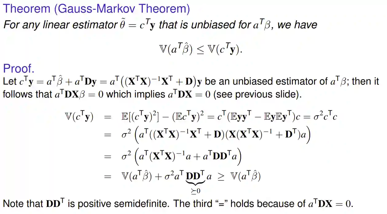
If we consider another estimator $\hat{\theta} = c^{T}y = a^{T}\hat{\beta} + a^{T}Dy$ we cannot use any deviation D, because if it is unbiased we will have $a^{T}DX = 0$

You can see the proof in the image: «««< HEAD This shows that among all the unbiased models MLE with ordinary least squares produces the best results, but some biased results could do better!

Regression is biased 🟥+

One can show that there are many examples where linear regression is quite biased. This is a problem especially with high dimensional data. There are some numerical instabilities with correlated features, especially when we are trying to invert something small (floating point imprecisions!)

6c2f795 (vault(): 2024-10-20 12:22:26)

Bias Variance trade-off 🟩

We want to decompose the value $\mathbb{E}_{D}\mathbb{E}_{X, Y}[(\hat{f}(x) - y)^{2}]$ where $f$ is the parameterised function that we are trying to learn, and $y$ is the true label. $D$ is our dataset is a distribution on all available datasets, and has an influence on $\hat{f}$ in this case., and $X, Y$ are the true un-accessible distributions of the data. Now let’s do some calculations. Let’s consider the value $\hat{y} = \mathbb{E}_{Y}[Y \mid X=x]$. Then let’s decompose the prediction error at $X = x$

$$ \mathbb{E}_{D}\mathbb{E}_{Y\mid X=x}[(\hat{f}(x) - \hat{y} + \hat{y} - y)^{2}] = \mathbb{E}_{D}\mathbb{E}_{Y\mid X=x}[(\hat{f}(x) - \hat{y})^{2}] + \mathbb{E}_{D}\mathbb{E}_{Y\mid X=x}[(\hat{y} - y)^{2}] + 0 $$

Now $\mathbb{E}_{D}\mathbb{E}_{Y\mid X=x}[(\hat{y} - y)^{2}] = \mathbb{E}_{Y \mid X=x}[(\hat{y} - y)^{2}]$ because we are not training anything on $D$, and one can see that this is the noise variance, mean difference between the correct mean and the $y$ itself.

Now we further decompose the formulas

$$ \mathbb{E}_{D}\mathbb{E}_{Y\mid X=x}[(\hat{f}(x) - \hat{y})^{2}] = \mathbb{E}_{D}\mathbb{E}_{Y\mid X=x}[(\hat{f}(x) - \mathbb{E}[\hat{f}(x)] + \mathbb{E}[\hat{f}(x)]- \hat{y})^{2}] = \mathbb{E}_{D}[(\hat{f}(x) - \mathbb{E}[\hat{f}(x)])^{2}] + \mathbb{E}_{D}[( \mathbb{E}[\hat{f}(x)] - \hat{y})^{2}] + 0 $$

The first term - $\mathbb{E}_{D}[(\hat{f}(x) - \mathbb{E}[\hat{f}(x)])^{2}]$ - is the variance, the second term simplifies to $( \mathbb{E}[\hat{f}(x)] - \hat{y})^{2}$ as everything is constant with respect to $D$ inside that, this is the bias squared (the expected prediction model across all possible datasets minus the expected real value).

Regularizers

A link to statistical learning 🟩

Quite often it is true that the Statistical learning framework with a cost function and a regularizator is exactly the same as a Maximum a posteriori estimate in the bayesian setting, we can see it quite quickly:

$$ \arg \min_{\theta} \sum_{n = 1}^{N} \mathcal{L}(f(x), y) + R(\theta) = \arg \max_{\theta} \prod_{i =1 }^{N} P(y \mid x, \theta) P(\theta) $$

If $R(\theta) = -\log(P(\theta))$ and $\mathcal{L}(f(x), y) = -\log(P(y \mid x, \theta))$, so we can see the prior as if it was a regularizer!

From a purely theoretical point of view, what we would like to calculate is the following $f^{*}(x) = \mathbb{E}_{Y \mid X} [Y \mid X = x]$, but the number of samples for each $x$ is sparse, quite often we don’t have a label for a specific $x$. We need a function assumption that uses the nearby samples to make inference of the points close to those. For Buhmann, model free is non sense because its just a hidden model.

Ridge regression 🟩–

With linear regression we assume that $y \approx w^{T}x = f(x;w) = f_{w}(x)$. And usually we have some regularization thing that prevents the overfitting.

For example a loss function could be:

$$ \hat{w} = \arg \min_{w\in \mathbb{R}^{d}} \sum_{i = 1}^{n} (y_{i} - w^{T}x_{i})^{2} + \lambda \lVert w \rVert ^{2}_{2} $$

This is called ridge regression. The penalty term makes the weights shrunk towards zero. This idea is also used in neural networks, where it is known as weight decay.

The ridge solutions are not equivariant under scaling of the inputs, and one should standardize the inputs before solving

With this function we have an analytical solution which is

$$ \hat{w} = (X^{T}X + \lambda I)^{-1} X^{T}y $$

It’s easy to derive this formula, just take the derivative with respect to $w$, just need to handle the vector calculus well enough. We note that adding the term on the diagonal of $X^{T}X$ makes the matrix non-singular which allows inversion. This was the original reason why it was introduced. Similar thing can be done with standard regression. We will later discover that this is somewhat equivalent to a MAP estimate in the bayesian learning setting, while the MLE estimate is the classical linear regression, see Bayesian Linear Regression.

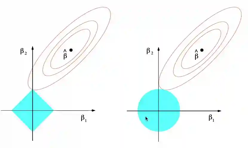
For Ridge to have a sparse solution, the best solution should be on one of the axis, which is rare, not for the Lasso! The lasso sparse solution region scales quadratically with the distance to the rombus, so it’s far more probable to have sparsity! This is very good for interpretability.

Lasso regression 🟩

The loss for the lasso is the following:

$$ \hat{w} = \arg \min_{w\in \mathbb{R}^{d}} \sum_{i = 1}^{n} (y_{i} - w^{T}x_{i})^{2} + \lambda \lVert w \rVert_{1} $$

Which is without the power of two (just sum of the values norm) $\lVert w \rVert_{1} = \sum_{i =1}^{d} \lvert w_{i} \rvert$

This is equivalent to the bayesian view with a special prior on the weights

$$ w \sim \frac{\lambda}{4\sigma^{2}}\exp\left( -\lvert w \rvert \frac{\lambda}{-2\sigma^{2}} \right) $$

Which is a Laplace distribution.

This is an image from the ESLI book. It justifies why with LASSO regularizers its far more easier to get sparse solutions. Diamonds are more likely to hit the error countours.

The Kernel Case 🟥

We have $x_{1}, \dots, x_{d} \in \mathbb{R}^{d}$ our feature functions. Let’s say we are trying to compute this feature function loss

$$ \hat{\beta} = \arg \min_{\beta \in \mathbb{R}^{\infty}} \sum_{i} (y_{i} - \beta^{T}\varphi(x))^{2} $$

The solution is the following using some calculus (same as normal equation solution).

$$ \hat{\beta} = (\Phi^{T}\Phi)^{-1}\Phi^{T}y $$

But this is impossible to compute because $\Phi$ is a matrix in $\mathbb{R}^{n \times \infty}$, but if we sneak in a $\Phi \Phi^{T}(\Phi \Phi^{T})^{-1}$. Then it simplifies to

$$ \hat{\beta} = \Phi^{T}(\Phi \Phi^{T})^{-1}y $$

Which simplifies a little bit because that $\Phi \Phi^{T}$ is a $\mathbb{R}^{n\times n}$ matrix, but we still need to solve the outside $\Phi^{T}$.

But it doesn’t matter during inference, because for inference we have

$$ \varphi(\hat{x})^{T}\hat{\beta} = \varphi(\hat{x})^{T}\Phi^{T}(\Phi \Phi^{T})^{-1}y $$

And the value $\varphi(\hat{x})^{T}\Phi^{T}$ which is just $\varphi(\hat{x})^{T} \varphi(x_{i}) = k_{i}(x)$ We can conclude and say

$$ \hat{\psi}(x) = k(x)A^{-1}y $$

With $A = \Phi \Phi^{T}$ the kernel matrix, where $A_{ij} = \varphi(x_{i})^{T}\varphi(x_{j})$.

But $A^{-1}$ is highly instable! This is why we add something in the diagonal, something similar to the ridge regression.

So we just add the thing on the diagonal: $\hat{\psi}(x) = k(x)(A + \lambda I)^{-1}y$

The classification Case

There is an analogous problem setting, but we assume that our target, the $y$ is some categorical data. So we still have the training dataset $\left\{ x_{i}, y_{i} \right\}_{i \leq n} \in \mathbb{R}^{d} \times \mathcal{Y}$, we need to find (learn) a function $f: \mathbb{R}^{d} \to \mathcal{Y}$. Usually $\mathcal{Y} = \left\{ 0, 1 \right\}$ or $\left\{ -1, 1 \right\}$. Some common assumptions for this problem settings are:

• $X \mid Y = y_{i} \sim \mathcal{N}(\mu_{i}, \Sigma)$ and unknown mean and variance
• $Y \sim \text{ Bern(0.5)}$ which is just uniform over the possible cases I think.

With those assumptions and using Bayes rule one can prove that the solution is

$$ P(y_{i} = 1 \mid X) = \sigma(\beta^{T}x) $$

Where $\beta$ is dependent on the mean and variance of the training samples. You should also take a look at Logistic Regression where we have a natural derivation of the Sigmoid function.

Ensemble methods

Some mean of methods have a more accurate prediction power. Let’s consider a set of estimators $f_{1}, \dots, f_{M}$, and their simple average defined as

$$ \hat{f}(x) = \frac{1}{M}\sum_{m = 1}^{M} f_{m}(x) $$

Then the bias is

$$ \text{ bias }[\hat{f}(x)] = \mathbb{E}_{D}[\hat{f}(x)] - \mathbb{E}[Y\mid X=x] = \frac{1}{M}\sum_{m = 1}^{M} \mathbb{E}_{D}[f_{m}(x)] - \mathbb{E}[Y\mid X=x] = \frac{1}{M} \sum_{m=1}^{M}bias(\hat{f}_{m}(x)) $$

Which implies if we have unbiased estimators, the ensemble will also be unbiased.

If we look at the variance we will see that

$$ \text{Var}[\hat{f}(x)] = \frac{1}{M^{2}}\sum_{m = 1}^{M} \text{Var}[f_{m}(x)] + \frac{1}{M^{2}}\sum_{m \neq l} \text{Cov}[f_{m}(x), f_{l}(x)] $$

And if the covariance is small enough, then the variance of the ensemble is smaller than the variance of the individual estimators, which is why the wisdom of the crowds work. We gain variance reduction of $\frac{\sigma^{2}}{M}$

References

[1] Hastie et al. “The Elements of Statistical Learning: Data Mining, Inference, and Prediction, Second Edition” Springer Science & Business Media 2009