3D representations

In this section, we present some of the most common 3D representations used in computer graphics and computer vision. Each representation has its own advantages and disadvantages, and the choice of representation often depends on the specific application.

Voxels

With voxels we discretize 3D space into a 3d grid, it is an intuitive manner to represent the data, but it has limited resolution. It needs $\mathcal{O}(n^{3})$ memory.

Points and Volumetric primitives

We can discretize surfaces into 3D points. Yet, this does not model connectivity, and might vary from frame to frame if it is a video.

Many hardware cameras (like LiDAR) use this representation, and it is also used in some 3D reconstruction methods.

Meshes

We discretize vertices and faces, we know about connectivity. GPUs were made to handle this kind of data for example. Yet we have a limited number of vertices and faces (fixed resolution, which means we have an approximation error). Unreal Engine 5 Nanite has a way to decide when to use more triangles (more detail), or less (example long fields). Usually most fine-grained description is around one triangle per pixel (more is useless, you cannot render it). But as scientists, we like to represent it as continuous functions.

Implicit Representations

We can represent surfaces as the level-set of a continuous function => We have arbitrary topologies (for intro to topology see Topological Spaces). We use neural networks to approximate these implicit functions and shapes. Many many complex shapes can be represented with these implicit functions, but they need to be converted to representations above to be visualized.

Signal Distance Fields (SDF)

Normally, SDF (signal distance field $f_{\theta} : \mathbb{R}^{3} \times \mathcal{X} \to R$) values are stored in a grid (this is quite memory consuming), meaning every cell stores the signed distance from the surface (negative means inside, positive means outside).

Neural Implicit Representations

Here we have neural networks that represent space information (if the shape is inside or outside).

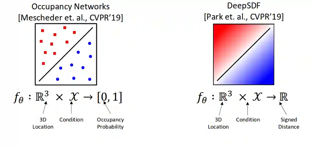
Two representations - Occupancy Networks and DeepSDF

We use simple MLP (see Neural Networks) to represent these images.

• Occupancy networks are just classification problems (you sample points, and decide if a point is inside or outside).

• DeepSDF is a regression problem, you sample points and predict the signed distance from the surface (you find level sets to know the surface).

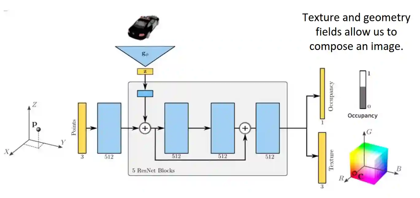
The other idea is that we can use these neural fields also for color, lighting, radiance, and similar things (meaning more information)! Another nice thing is that normals are **gradients of the level set**, during backpropagation we have this information for free. The only problem when the translation to meshes happens is that at vertices, the normals are not well defined.

Marching Cubes

This is a rendering technique.

Marching Cubes can extract renderable meshes from these implicit shapes, it is a way to convert the implicit representation to a mesh. This looks like a good web resource to give a brief idea of the method. It divides the space into voxels, and queries for inside and outside for the vertices, after it gets the configuration of the inside outside, it can render some triangles for the mesh.

Learning Implicit Shapes

This section explores most common ways to learn the implicit representations mentioned above.

Watertight meshes

We can create some sort of a surrogate model after having a first easily renderable (but more memory costly model) in the following way:

• With these kinds of meshes we sample 3D points in space
• we query occupancy to the model (this is some ground value).
• After creating this dataset, then you can use a cross entropy loss to train the implicit shape.

$$ \mathcal{L}(\theta, \phi) = \sum_{j = 1}^{K} \text{BCE}(f_{\theta}(p_{ij}, z_{i}), o_{ij}) $$

Where $\text{BCE}$ is the binary cross entropy, $f_{\theta}$ is the implicit function, $p_{ij}$ are the sampled points, $z_{i}$ are the latent variables (if you have some), and $o_{ij}$ are the occupancy labels (inside or outside).

Learning from Points

See this paper -> (Gropp et al. 2020). The main problem with this format is that we have no connectivity information, and we need to learn it from the data. For example if you have some points in a circle, it is not obvious to define whether if a points is actually inside or outside the circle.

For example, both of the following solutions are plausible:

$$ \lVert \nabla f_{\theta}(\boldsymbol{x}) \rVert_{2} = 1 $$

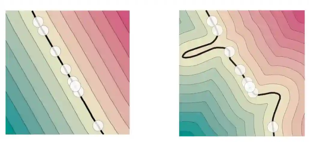
We won’t explain the maths behind this, but it is a way to enforce the model to learn the distance field.

$$ \mathcal{L}(\theta) = \sum_{i \in I} \lvert f_{\theta}(\boldsymbol{x}_{i}) \rvert^{2} + \lambda \sum_{j \in J} \left( \lVert \nabla f_{\theta}(\boldsymbol{x}_{j}) \rVert_{2} - 1\right)^{2} $$

This was introduced from a paper in 2020 cited above.

Learning from Images

The following is the general idea of this technique:

• We usually have video from 2D images.
• We model geometry and appearance with neural implicit fields.
• We can use a differentiable renderer to render the images, and then optimize the parameters of the implicit field with a loss function that compares the rendered images with the original ones. Once you have this renderer trained, we can use it to render new images from different viewpoints.

Forward Rendering

How can we develop a differentiable rendering engine? From the camera point, we shoot the ray for all pixels $\boldsymbol{u}$ and render using the predicted occupancy and texture data, using the texture field at the found point. (To find intersection they use root finding, also called secant method).

Secant Root Method

$$ f_{\theta}(x_{j}) < \tau \leq f_{\theta}(x_{j+1}) $$

Then you can use the description of the algorithm above and do it several times until it converges to the value.

Backward pass

The idea is now we have a rendering, we can have an image back and compare it with the original.

• Image Observation $\mathbf{\hat{I}}$
• Loss: $\mathcal{L}(\hat{\mathbf{I}}, \mathbf{I}) = \sum_{\mathbf{u}} \| \hat{\mathbf{I}}_{\mathbf{u}} - \mathbf{I}_{\mathbf{u}} \|$
• Gradient of loss function

$$ \begin{align*} \frac{\partial \mathcal{L}}{\partial \theta} &= \sum_{\mathbf{u}} \frac{\partial \mathcal{L}}{\partial \hat{\mathbf{I}}_{\mathbf{u}}} \cdot \frac{\partial \hat{\mathbf{I}}_{\mathbf{u}}}{\partial \theta} \\ \frac{\partial \hat{\mathbf{I}}_{\mathbf{u}}}{\partial \theta} &= \frac{\partial t_\theta(\hat{\mathbf{p}})}{\partial \theta} + \frac{\partial t_\theta(\hat{\mathbf{p}})}{\partial \hat{\mathbf{p}}} \cdot \frac{\partial \hat{\mathbf{p}}}{\partial \theta} \end{align*} $$

Differentiation of $\frac{\partial \hat{\mathbf{p}}}{\partial \theta}$ is tricky because $\hat{\mathbf{p}}$ is only implicitly defined and found iteratively via the Secant method. You can find an analytic solution for $p$ so that also that part is differentiable. Consider the ray: $\hat{\mathbf{p}} = \mathbf{r}_0 + \hat{d} \mathbf{w}$

Condition for surface-ray intersection: $f_\theta(\hat{\mathbf{p}}) = \tau$

Implicit differentiation on both sides with respect to $\theta$:

$$ \frac{\partial f_\theta(\hat{\mathbf{p}})}{\partial \theta} + \frac{\partial f_\theta(\hat{\mathbf{p}})}{\partial \hat{\mathbf{p}}} \cdot \frac{\partial \hat{\mathbf{p}}}{\partial \theta} = 0 $$

Substitute $\hat{\mathbf{p}} = \mathbf{r}_0 + \hat{d} \mathbf{w}$:

$$ \frac{\partial f_\theta(\hat{\mathbf{p}})}{\partial \theta} + \frac{\partial f_\theta(\hat{\mathbf{p}})}{\partial \hat{\mathbf{p}}} \cdot \mathbf{w} \frac{\partial \hat{d}}{\partial \theta} = 0 $$

Solve for $\frac{\partial \hat{d}}{\partial \theta}$:

$$ \frac{\partial \hat{\mathbf{p}}}{\partial \theta} = \mathbf{w} \frac{\partial \hat{d}}{\partial \theta} = -\mathbf{w} \left(\frac{\partial f_\theta(\hat{\mathbf{p}})}{\partial \hat{\mathbf{p}}} \cdot \mathbf{w} \right)^{-1} \frac{\partial f_\theta(\hat{\mathbf{p}})}{\partial \theta} $$

We leave out the implementation details, the nice thing is that this is analytical.

Neural Radiance Fields

Neural Radiance Fields (NeRF) is a method for representing 3D scenes using neural networks. It is particularly useful for rendering novel views of a scene from a sparse set of input images. The view can have a drastic change in appearance, NeRF is a solution that attacks this kind of problems.

Introduction to NeRF

NeRF starts with a set of different views of a scene. For every scene it sends a ray and samples some points, getting its RGB value for every point and integrating. Then you combine this information from multiple views to create the final scene.

We add parameters of the viewing direction to the fully connected network, so we can have a different output for different viewing directions, and we also output the density value of the point.

Alpha Compositing

Alpha compositing is a technique used to combine images with transparency. In the context of NeRF, it is used to blend the colors of sampled points along a ray to produce the final pixel color. If a point has a high density, it means the alpha value is quite high (probaby the ray ends there).

$$ \begin{align*} \text{Alpha}: & \alpha_{i} = 1 - e^{-\sigma_{i} \delta_{i}}, \delta_{i} = \| \mathbf{p}_{i} - \mathbf{p}_{i-1} \|_{2} \\ \text{Transmittance}: & T_{i} = e^{-\sum_{j=1}^{i-1} \sigma_{j} \delta_{j}} \\ \text{Color}: & C_{i} = \mathbf{c}_{i} \cdot T_{i} \cdot \alpha_{i} \\ \end{align*} $$

There is a big cost in adding these samples, one way to make it cheaper is hierarchical sampling, to sample it more coarsely, and just taking into account where weights are high.

Training NeRF

Also NeRF use the image reconstruction as its loss (like image implicit shape rendering approach). The thing is that we have view information, and this can be combined to create a good representation of the static scene.

Positional Encoding with Fourier Features

These are the same features we have seen in Gaussian Processes when making them run faster, also similar with positional encodings in Transformers. This is needed since NN are biased towards learning lower frequency functions (I currently don’t know why this is true).

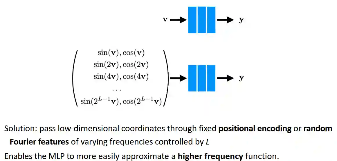Low and high frequency is also the same idea used for JPEG image format compression techniques.

Some forms of parameterization

Quick Small Volume Rendering We said that NeRF wastes a lot of computation when doing Alpha Compositing. The idea is to make smaller volumes close to the figure that we want to approximate. This makes that part more efficient, but you need to first describe the volumes (problem is shifted to another domain, usually you don’t have the volumes).

Spherical Primitives Instead of using pixels, we can use spheres, which are well supported by existing cuda kernels. The problem is that with sphere based reconstruction sometimes it is hard to have high quality for thin structures.

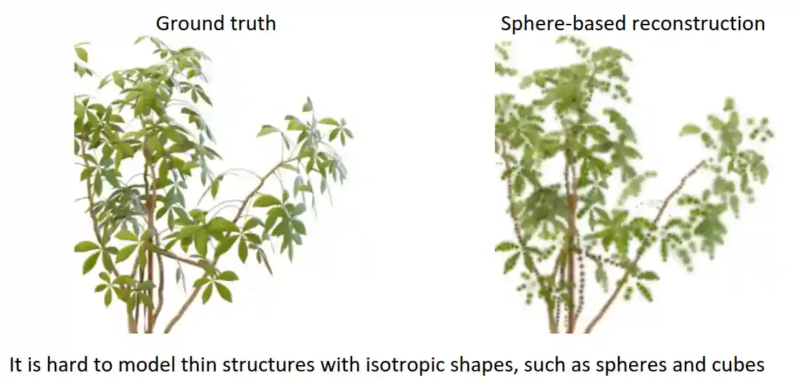
But this can be solved with elipsoid primitives, which are more flexible and can represent thin structures better.

Strenghts and weaknesses

• Strengths:

  • Can render novel views of a scene from a sparse set of input images.
  • Can handle complex lighting and reflections.
  • Can produce high-quality images with realistic details.
    • NeRF is a more flexible representation compared to implicit representation, since it has information about transparency and thin structure.

• Weaknesses:

  • Requires a large amount of calibrated views to train and render a scene effectively.
  • Slow rendering times, especially for high-resolution images.
  • Not suitable for dynamic scenes (NeRF is designed for static scenes).
  • Can produce artifacts such as floating objects or worse geometry compared to explicit representations like meshes.
  • Doesn’t produce a geometry that can be easily manipulated or edited, it has lots of noise, floaters compared to implicit surfaces. So this method is good if you want nice static images.

3D Gaussian splatting

This technique has been proposed in 2023, and has been quite influential now.

It is a method for representing 3D scenes using Gaussian splats, which are 3D Gaussian distributions that can be rendered efficiently. It is particularly useful for rendering novel views of a scene from a sparse set of input images.

One of their main advantages is fast inference.

• No MLP evaluation
• No ray marching or point sampling
• Almost real time 60fps rendering.
• Able to represent thin structures, NeRFs have problems with those.

Overview of the Technique

3D Gaussian splatting (See (Kerbl et al. 2023)) works by representing a scene as a collection of 3D Gaussian distributions, each with its own position, color, and opacity. These Gaussians can be rendered efficiently using GPU acceleration, allowing for real-time rendering of complex scenes.

Adaptive density control is used to add more detail to areas of the scene that require it, while reducing detail in areas that do not. This allows for efficient rendering without sacrificing quality. Examples are removing (if transparency is too low) or adding some Gaussians

• Under reconstruction: if you cannot fit the shape well, you add a gaussian, and then use the gradient information to fill the loss function
• over reconstruction: remove the gaussian (probably if the gradient is too low, at the end this is the signal.).

The gradient is the signal used to decide how to add or remove new Gaussians.

The Model

Gaussian Splatting uses 3D gaussian primitives. Each Gaussian has four parts:

1. A center $\mu \in \mathbb{R}^{3}$
2. A covariance matrix $\Sigma \in \mathbb{R}^{3 \times 3}$, often expressed as rotation and diagonal scaling to maintain positive semi-definitivenes $\Sigma = RSS^{T}R^{T}$.
3. Color $c \in \mathbb{R}^{3}$, sometimes replaced with spherical harmonics $\in \mathbb{R}^{9}$ especially for view dependent formats.
4. And an opacity value $o \in\mathbb{R}$.

Rendering with Gaussian Splatting

We only consider Gaussians close to the point in2D space, sort it in vicinance order with GPU (so O(n) sorts), and then use alpha compositing to render the scene.

$$ \alpha = o \cdot \exp(-0.5 (x - \mu')^{T}\Sigma^{'-1}(x- \mu')) $$$$ C = \sum_{i} \alpha_{i} c_{i} \prod_{j=0}^{i-1} (1 - \alpha_{j}) $$

The main difference is that here we use Gaussians instead of MLPs, and we can render them in parallel (makes this very fast).

Applications in Human Body Reconstruction

This theme is important for the lab that is giving the course, also take a look at Parametric Human Body Models.

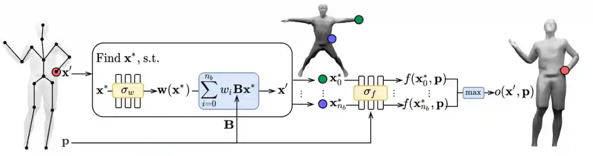
SNARF

We have 3D meshes, and we map it to a canonical pose (also called star pose). Then you compute the skinning weights to pose the implicit shape to unseen poses, now you can animate it to new poses, which is a quite cool industry application.

The difficult part is how to map the starting image to the canonical space. The idea here is to predict skinning weights, and use pose parameters to check if it matches the canonical pose or not. This is called forward warping.

Vid2Avatar

From single monocular video we can:

• Reconstruct geometry
• Separate human from background
• Reconstruct human’s appearance.

The main point here is that you can use the ideas above to make these beautiful reconstructions.

Multi-View Reconstruction and Tracking

If you attach some Gaussians to some meshes, you can track how the object moves, this is the basic idea. They show you can keep tracking the movement also after drastic changes!

References

[1] Gropp et al. “Implicit Geometric Regularization for Learning Shapes” PMLR 2020

[2] Kerbl et al. “3D Gaussian Splatting for Real-Time Radiance Field Rendering” arXiv preprint arXiv:2308.04079 2023