Introduction: a neuron

I am lazy, so I’m skipping the introduction for this set of notes. Look at Andrew Ng’s Coursera course for this part (here are the notes). Historical paper is (Rosenblatt 1958). One can view a perceptron to be a Log Linear Models with the temperature of the softmax that goes to 0 (so that it is an argmax). Trained with a stochastic gradient descent with a batch of 1 (this is called the perceptron update rule, see The Perceptron Model).

Structure of a neuron

Artificial neurons, though inspired by biological neurons (see The Neuron), are not exact replicas. There are key differences:

• Biological neurons encode time information between their spikes.
• They do not spike in a forward clean order, but have recurrent feedbacks that in ANN often are not modelled.
• They are a lot more energy efficient compared to ANN.

Mathematical description

A single layer of a function can be written in the following way:

$$ F(\theta)(x) = \phi(Wx + b) $$

Which can be summarized by: linear part + activation function. Where $F(\theta)$ is a partial function that returns another function, $\theta = (W, b)$ a vector, this is just a way to separate the bias with the parameters. The $\phi$ is the non linearity, that is needed for the universal approximation function.

Compositionality

The main idea in going deep is extract features of increasing complexity, it’s like attempting to give it more computation so that it is possible to extract more interesting parts. We can mathematically view deep networks in the following way:

$$ x = F^{(l)} F^{(l - 1)} \dots F^{(0)}(x_{0}) $$

And a composition of layers!

Modularity

We can compose parts of the network together! For example residual networks are a clear example, or the inception network.

Universal approximation theorem

This theorem states that neural networks can approximate any continuous function to arbitrary precision. The idea is just using a single layer with a non-linear activation function to write level sets. The proof is here (Hornik et al. 1989). This is a nice interactive website that proves it: here.

More formally: Let $\sigma: \mathbb{R} \rightarrow \mathbb{R}$ be a non-constant, bounded and continuous (activation) function $I_m$ denotes the $m$-dimensional unit hypercube $[0,1]^m$ and the space of real-valued functions on $I_m$ is denoted with $C(I_m)$.

Then any function $f \in C(I_m)$ can be approximated given any $\epsilon > 0$, integer $N$, real constants $v_i, b_i \in \mathbb{R}$ and real vectors $\mathbf{w}_i \in \mathbb{R}^m$ for $i = 1, \dots, N$:

$$ f(\mathbf{x}) \approx g(\mathbf{x}) = \sum_{i=1}^{N} v_i \sigma(\mathbf{w}_i^T \mathbf{x} + b_i) $$

And: $|g(\mathbf{x}) - f(\mathbf{x})| < \epsilon$ , for all $\mathbf{x} \in I_m$

Hopfield Networks

Hopfield networks are a type of recurrent neural network that can store and retrieve patterns. They are particularly useful for associative memory tasks, where the network can recall a stored pattern given a noisy or partial input.

The Hopfield Network Model

$$ \Theta = \sum_{i = 1}^{s} \left[ x_{t}x_{t}^{T} - \boldsymbol{I}_{n} \right] $$

One can prove that this matrix is symmetric, and that it is irreflexive (meaning $\forall j: \Theta_{jj} = 0$).

The update Rule

The state of each neuron can be either 0 or 1, and the network evolves over time according to the following update rule:

$$ x_{t + 1} = \begin{cases} \text{sign}(\Theta x_{t}) & \text{ if } \Theta x_{t} \neq 0 \\ x_{t} & \text{ if } \Theta x_{t} = 0 \end{cases} $$

Training network tricks

Activation functions

Solitamente le funzioni classiche per i network neurali sono sigmoid, tanh, e ReLU. La cosa brutta delle prime due è vanishing gradient, perché se il valore è molto grosso o molto piccolo, la derivata è molto vicino allo 0, quindi è molto difficile aggiornare.

The activation function is presented as $\phi$ before. One thing to note is that this non-linearity doesn’t mix the dimensions together. Let me explain clearly with some maths:

We say that $\phi: \mathbb{R}^{n} \to \mathbb{R}^{n}$ and it’s a composition of some $\bar{\phi}: \mathbb{R} \to \mathbb{R}$ which are just applied independently to every dimension.

Other properties are:

• Increasing
• Continuous There are important to remember from a mathematical point of view.

Level Sets

$$ L_{f}(z) = \left\{ x : \phi(w\cdot x + \beta) = z \right\} \perp w $$

These are also called generalized linear models, or ridge functions.

ReLU activation

$$ f(x) = \begin{cases} 0,\, \text{ if } x < 0 \\ x, \, \text{ if } x \geq 0 \end{cases} $$

The important thing to notice is that when it backpropagates, it just activates or kills the signal, allowing the gradient to flow naturally, and not vanish.

$$ \frac{ \partial x^{(k+1)} }{ \partial x^{(k)} } = \sigma'(W^{(k)}x^{(k)} + b) W^{(k)} $$

And $\sigma'$ in the case of the ReLU is just 0 or 1, which aids toward the problem of vanishing gradient and similars. The thing to note is that this doesn’t exactly work as an activation function if the input depends on $x$ with more than one parameter

Hyperbolic tangent

This activation is usually preferred to the Sigmoid, better treated in Logistic Regression, because it has sign symmetry.

Importance of Non linearity

The main reason we need non linearity is that we want to be able to learn complex functions, and this is not possible with a linear function. We can see this by the fact that a composition of linear functions is still a linear function.

Let’s analyze the topic mathematically: Suppose you have input data $x \in \mathbb{R}^{n}$ and a function $\sigma : \mathbb{R}^{n} \to \mathbb{R}^{n}: \sigma(x) = \alpha x + \beta$, the problem is the if you nest layers: $\forall l \in \left[ 1, L \right], x^{[l]} = \alpha(W^{[l]} x^{l - 1}] + b^{[l]}) + \beta$ which is just another affine mapping. This means all the layers are the same as if I used a single layer. Using Kernel Methods could help in this case, but it often needs feature engineering which is done by humans.

Optimization

Momentum, praticamente un gradient descent che tiene conto delle computazioni passate, e calcola la direzione anche secondo quelle (quindi se vado su e giù e a destra sempre nelle iterazioni passate, andrò a destra più spesso diciamo, questa è l’intuizione per questa idea).

Una cosa molto strana è che il training delle NN è molto stabile. Cioè vari un pò l’input e non varia molto l’ouput!

Possibili motivi:

1. Weights
2. Loss function
3. Internal redundancy? cioè ho troppi parametri e questo lo rende bello.(teoria del prof)

Loss functions

$$ \mathcal{l}(y, \hat{y}) = \frac{1}{2} \lVert y - \hat{y} \rVert ^{2} $$$$ l(\theta)(x, y) = l(y, F(\theta)(x)) $$

Sometimes you need to tailor the loss function to the problem you are trying to solve! For example a very famous function is the Softmax Function, for multiclass classification. In the case you just have two classes then it’s the logistic function.

$$ l(y, \hat{p}) = - \log \hat{p}_{y} $$

If we view this from an information theoretical point of view, then it’s the expected length of our codeword.

Risks

After we have the loss we can go on and define the empirical risk, which is just:

$$ \mathcal{R}(\theta; \mathcal{S}) := \mathbb{E}_{\mathcal{S}} [\ell(\theta)] := \frac{1}{s} \sum_{i = 1}^{s} \ell(\theta)(x_{i}, y_{i}) = \frac{1}{s} \sum_{i = 1}^{s} \ell(y_{i}, F(\theta)(x_{i})) $$

This is the training risk, and same thing could be defined for the test risk.

Quirks of Neural Networks

This section presents some counter-intuitive phenomena that pertain neural networks. Classical theories predict opposite behaviours compared the ones we list here.

Grokking

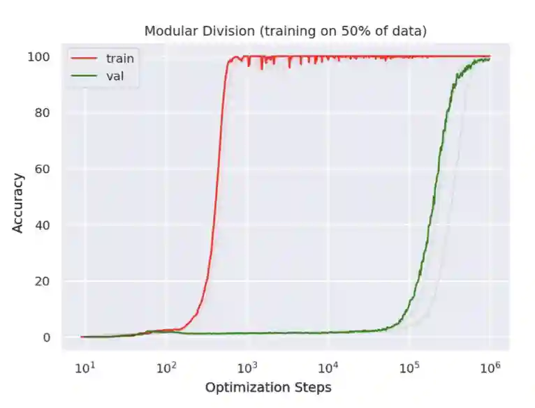
Grokking refers to the phenomenon where a neural network initially exhibits poor generalization despite achieving low training loss, but after extended training, it suddenly generalizes well without any further changes to the dataset or training procedure. This phenomenon was first observed in algorithmic tasks, where models would first memorize the training data before gradually developing a more structured, generalizable understanding.

This delayed phase transition challenges conventional notions of overfitting and suggests that prolonged training on sufficiently large datasets can sometimes lead to emergent generalization. A possible explanation is that neural networks first fit simpler patterns before refining their internal representations to capture deeper structure.

Double Descent

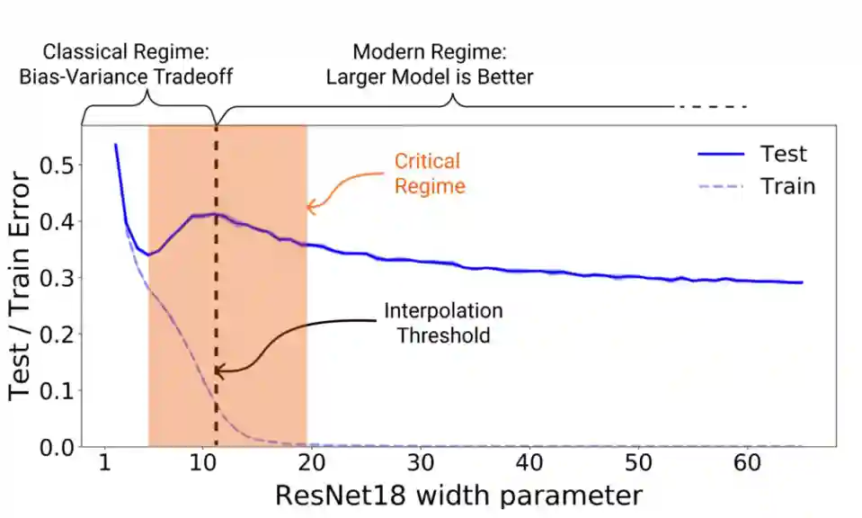
The double descent phenomenon describes a peculiar behavior in the generalization performance of neural networks as model capacity increases. Unlike classical machine learning theory, which suggests that increasing model complexity leads to overfitting beyond a certain point, double descent reveals a second improvement in generalization performance at very high capacity.

This behavior is characterized by two distinct regions:

1. Classical Bias-Variance Tradeoff: In the underparameterized regime, increasing model complexity improves performance until it reaches the interpolation threshold, where it perfectly fits the training data but generalizes poorly.
2. Modern Overparameterization: Beyond this interpolation threshold, further increasing model capacity counterintuitively leads to improved generalization. Neural networks often enter this second descent phase, where overfitting seems to subside, and test performance improves.

The authors define a measure of Effective Model Complexity (EMC) as the maximum number of samples that can be memorized by the model, and make an analysis with this. They show that in some specific cases it hurts to have more data, as more data shifts the critical regime to the right.

Label Memorization

Neural networks have a remarkable capacity to memorize training data, even when the labels are randomized. Studies show that deep models can fit arbitrary labels, suggesting that memorization is an inherent property rather than a failure of training. However, memorization does not necessarily contradict generalization: modern deep networks balance memorization with pattern recognition.

Key insights into label memorization include:

• Memorization is a function of dataset size and model capacity: Larger networks can store training examples verbatim, but this does not always harm test accuracy, particularly in large-scale training scenarios.
• Memorization and generalization can coexist: Empirical results suggest that networks first learn patterns present in the data before resorting to memorization for harder examples.

References

[1] Hornik et al. “Multilayer Feedforward Networks Are Universal Approximators” Vol. 2(5), pp. 359--366 1989

[2] Rosenblatt “The Perceptron: A Probabilistic Model for Information Storage and Organization in the Brain.” 1958