While Active Learning looks for the most informative points to recover a true underlying function, Bayesian Optimization is just interested to find the maximum of that function. In Bayesian Optimization, we ask for the best way to find sequentially a set of points $x_{1}, \dots, x_{n}$ to find $\max_{x \in \mathcal{X}} f(x)$ for a certain unknown function $f$. This is what the whole thing is about.
Definitions
First we will introduce some useful definitions in this context. These were also somewhat introduced in N-Bandit Problem, which is one of the classical optimization problems we can find in the literature.
We suppose there is an underlying function $f$, but we are only observing some noised estimates $y = f + \varepsilon$ where $\varepsilon$ is usually modeled as Gaussian noise.
At each time step we can choose some $x_{t}$, then the reward is $y_{t} = f(x_{t}) + \varepsilon_{t}$. We would like to maximize the cumulative reward $\sum_{t=1}^{n} y_{t}$.
Regret
$$ R_{n} = \sum_{t=1}^{n} f(x^{*}) - f(x_{t}) $$$$ \lim_{n \to \infty} \frac{R_{n}}{n} = 0 $$Intuitively, it says that if we explore enough, then we will always get the best possible choice.
Regret and maximum of the function
$$ \lim_{ n \to \infty } f(x_{n}) = \max_{x} f(x) \iff \lim_{ n \to \infty } \frac{R_{n}}{n} = 0 $$Proof:
Using Cesàro Mean we quickly verify the $\implies$ direction. For the inverse we see the following:
$$ \begin{align} \lim_{ n \to \infty } \frac{R_{n}}{n} &= \lim_{ n \to \infty } \frac{\left( \sum_{t = 1}^{n} \max_{x} f(x) - f(x_{t}) \right)}{n} \\ &= \max_{x}f(x) - \lim_{ n \to \infty } \frac{1}{n} \sum_{t = 1}^{n}f(x_{t}) \\ &\implies \lim_{ n \to \infty } \frac{1}{n} \sum_{t = 1}^{n}f(x_{t}) = \max_{x} f(x) \end{align} $$Then it follows from the other direction of the Cesàro mean.
Exploration and Exploitation
This setting naturally leads to the exploration-exploitation tradeoff. We can either choose to explore new regions of the input space, or exploit the regions we have already visited. It’s easy to observe that both greedy strategies that only exploit the current best guess and strategies that only explore new regions are not optimal, meaning they will yield not sub-linear regrets.
Optimization Techniques
A standard Idea
In the rest of the section, we will assume that the $f$ function is a Gaussian Process. Then one greedy way to solve this optimization problem is the following algorithm
- Initialize a $f \sim GP(\mu_{0}, k_{0})$.
- For $t = 1, \dots, n$ do
- Find the point $x_{t} = \arg\max_{x \in \mathcal{X}} f(x)$.
- Observe the reward $y_{t} = f(x_{t}) + \varepsilon_{t}$.
- Update the GP with the new observation.
On the need of Calibrated Models
The most important of the following models is the GP-UCB acquisition function that heavily relies on the calibration assumption. Recall Bayesian neural networks for a refresh on calibration. Intuitively, only in the case of calibrated models, the confidence bounds given by the GP relates to the accuracy of the prediction. If a model is not calibrated, the confidence doesn’t tell you anything on the accuracy of the prediction.
$$ \forall t \geq 1, \forall x \in \mathcal{X} : f^{*}(x) \in \mathcal{C}_{t}(x) = [\mu_{t}(x) - \beta_{t}\sigma_{t}(x), \mu_{t}(x) + \beta_{t}\sigma_{t}(x)] $$Which is the confidence interval defined by the GP-UCB algorithm.
Bound over confidence intervals
$$ \beta_{t}(\delta) \in \mathcal{O}(\sqrt{ \log(\lvert \mathcal{X} \rvert t / \delta ) }) $$Entropy Search
This method expands the d-optimality criteria, by looking for the point that gives the maximal information on the point we are looking for. There is a chicken and egg problem here, as the point itself.
GP-UCB
The idea
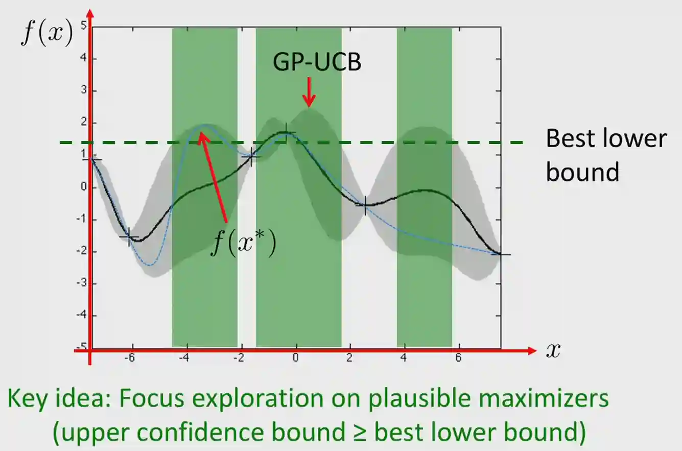
 Image taken from slides of the PAI course ETH 2024.
Optimism in the face of uncertainty
We just want to pick the point that maximizes our upper confidence bound in the posterior of the Gaussian Processes. The green region are the possible regions that we would like to sample from, as their upper confidence is higher than our lower bound. This idea is recurring in this setting.
If the model is well calibrated, then the uncertainty regions are coherent with what actually returns the underlying function. This motivates why we can safely ignore the zones on our input where the maximum is less than the minimum value of the variance. We are sure, due to calibration, that those zones do not contain our maximum with high confidence.
UCB Picking principle
$$ x_{t} = \arg\max_{x \in D} \mu_{t - 1}(x) + \beta_{t - 1} \sigma_{t - 1}(x) $$Where $\mu_{t - 1}(x)$ is the mean of the GP at the point $x$ and $\sigma_{t - 1}(x)$ is the standard deviation. $\beta_{t - 1}$ is a parameter that we can tune to have more or less exploration. This should select the point that maximizes the upper confidence bound in the GP.
We observe that if $\forall t,\beta_{t - 1} = 0$ then the algorithm is purely exploitative, while if $\beta_{t - 1} = \infty$ then the algorithm is purely esplorative, and it’s equivalent to uncertainty sampling presented in Active Learning.
The point can be found using standard one dimensional optimization techniques (e.g. random sampling or similars).
Convergence Bound on GP-UCP
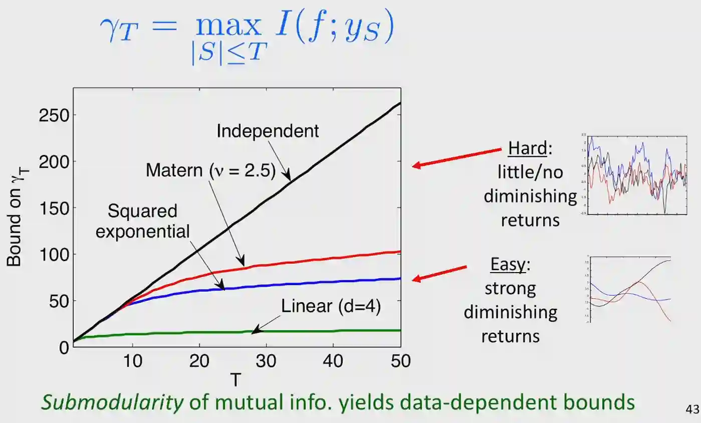
$$ \frac{1}{T} \sum_{t = 1}^{T} (f(x^{*}) - f(x_{t})) = \mathcal{O}\left( \sqrt{\frac{\gamma_{T}}{T}} \right) $$The maximum information gain determines the regret, often indicated as $\gamma_{T}$, sometimes as $\max_{S \leq T} I(f; y_{S})$. This sets the rate at which we get information. Due to submodularity of mutual information we can show that $\gamma_{T}$ can at most grow linearly with $T$.
I have no idea why this is true.
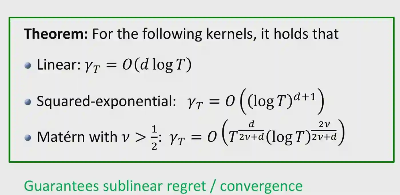
These are the bounds for different kernels in the GP
 The nice thing is that with all these kernels, we have guarantees that the regret is sub-linear, so we get the best possible solution.
And using the GP informational result from Active Learning we have:
$$ \begin{align} \frac{1}{T} R^{2}_{T} &\leq \sum_{t = 1}^{T}r_{t}^{2} \text{ Cauchy-Schwarz} \\ &\leq 4 \beta_{t}^{2} \sum_{t = 1}^{T} \sigma_{t}^{2}(x_{t}) \\ &= 4 \sigma_{n}^{2} \beta_{t}^{2} \sum_{t = 1}^{T} \frac{\sigma^{2}_{t}(x_{t})}{\sigma^{2}_{n}} \\ &\leq 4C \sigma_{n}^{2} \beta_{t}^{2} \sum_{t = 1}^{T} \log \left( 1 + \frac{\sigma^{2}_{t}(x_{t})}{\sigma^{2}_{n}} \right) \\ &= 4C \sigma_{n}^{2} \beta_{t}^{2} I(f_{T}; y_{T}) \in \mathcal{O}(\beta^{2}_{T}\gamma_{T}) \end{align} $$Growth rate of information gain
There is a clean intuition for the following graph: if the function is continuous, smooth so to say, then knowing the value of one point gives lots of insights to the value of the next point. Which means we need fewer point to get a good estimate of the function (this is why the slope of the function is low). If we have quite independent samples, then we need more points to get a good estimate of the function. This is why it has a linear growth rate: every point gives you about the same information. Note that this happens only for white noise, so probably it is not a much interesting case.

Choosing the point
Usually the acquisition function is non-convex, so we need some methods to compute that maximum.
- Low dimensionality: we can use lipschitz optimization.
- High dimensionality: we can use gradient descent.
Probability Improvement
The PI Idea
$$ I_{t}(x) = (f(x) - \hat{f}_{t})_{+} $$Where $\hat{f}$ is the current maximum. Then the point that is going to be picked is the point that maximizes the probability of having an improvement:
$$ x_{t + 1} = \arg \max_{x \in \mathcal{X}} \mathbb{P}(f(x) > \hat{f}_{t} \mid x_{1:t}, y_{1:t}) = \arg \max_{x \in \mathcal{X}} \Phi \left( \frac{\mu_{t}(x) - \hat{f}_{t}}{\sigma_{t}(x)} \right) $$We observe that this algorithm is a little biased towards exploration as it prefers large means with low variances.
Expected Improvement
$$ x_{t + 1} \arg \max_{x \in \mathcal{X}}\mathop{\mathbb{E}}[I_{t}(x) \mid x_{1:t}, y_{1:t}] $$It can be proven that Expected Improvement has the same regret bound as UCB. One drawback of this method, is that the optimization objective is usually flat, which makes it more difficult to optimize.
Thompson Sampling
Thompson Sampling Method
$$ f_{t + 1} \sim p( \cdot \mid x_{1:t}, y_{1:t}) $$And the find the new point as the maximum of this function $x_{t + 1} = \arg\max_{x \in \mathcal{X}} f_{t + 1}(x)$. In this case, we are leveraging the randomness of $f$ to trade between exploitation and exploration. Similar bounds to UCB can be established also for Thompson.
Information Directed Sampling
Regret Information Ratio
$$ \Psi_{t}(x) = \frac{\Delta(x)^{2}}{I_{t}(x)} $$Where $\Delta(x) = \max_{x'}f^{*}(x') - f^{*}(x)$ and $I_{t}$ is a function that captures the information gain (doesn’t need to be the same as the one for probability improvement).
Regret Bound for ID
$$ R_{T} \leq \sqrt{\sum_{t = 1}^{ T}I_{t - 1}(x_{t}) \cdot \sum_{t = 1}^{T} \Psi_{t - 1}(x_{t}) } $$ID Algorithm
$$ \hat{\Delta}_{t}(x) = \max_{x'\in \mathcal{X}} u_{t}(x') - l_{t}(x) $$Where $u$ and $l$ are respectively, the upper and lower bound for a calibrated model.
$$ x_{t + 1} = \arg \min _{x \in \mathcal{X}} \left( \frac{\hat{\Delta}_{t}(x)^{2}}{I_{t}(x)} \right) $$A common problem
One common problem with these methods is the kernel. How could we choose the correct kernel and its hyper-parameters? We are using these kernels to select the data itself, which could be quite biased; phrased in another manner: we are dependently selecting points based on the model (which is a good thing, but also the main drawback!) Another problem is getting calibrated models in this setting where you continuously select points. And often, datasets in this domain are quite small.
Common approaches to this problem are:
- Imposing priors on the kernel parameters.
- Occasionally selecting random points.