Active Learning concerns methods to decide how to sample the most useful information in a specific domain; how can you select the best sample for an unknown model? Gathering data is very costly, we would like to create some principled manner to choose the best data point to humanly label in order to have the best model.
In this setting, we are interested in the concept of usefulness of information. One of our main goals is to reduce uncertainty, thus, Entropy-based (mutual information) methods are often used. For example, we can use active learning to choose what samples needs to be labelled in order to have highest accuracy on the trained model, when labelling is costly.
Setting
Given a safe exploration space , an interesting space and all possible space and a dataset we want to find the best points that we would like to sample in to maximize the information we can get about .
So we want to collect the most representative sample under constrained budgeting.
We can divide the setting in Active Learning as solving two problems:
- Quantifying the concept of utility of a sample.
- Finding the best sample to select.
Utility of samples
One idea from Entropy is the concept of mutual Information: how much observing reduces the uncertainty of . It is defined as:
Information Gain in Linear Regression
This measures the gain of adding to the set for a certain function .
The result will be
Where and .
Marginal Gain
First we define the notion of marginal gain:
We write with where contains all possible points to mean:
Which is a mutual information for a lot a lot of points. Instead of writing the for all we can write .
There is a nice property of this Marginal Gain:
This relation will be quite important for the proof of submodularity of mutual information.
Submodularity of Mutual Information
Mutual Information is submodular, meaning it satisfies the following relationship: Given and :
Using the above definition of marginal gain, we can write this as:
This property just says that the gain of adding a point to a small set is higher than adding it to a bigger set.
Proof: We first notice that:
Which ends the proof .
Submodularity means no synergy
Remember from Entropy that synergy means between two random variables and means . We will prove now that the submodularity property is equivalent to absence of synergy between observations. We want to show that for all we have:
Proof:
Monotonicity of Information
One can prove that if then . This is a quick consequence on the monotonicity of Entropy explored in Entropy.
Greedy optimization
Uncertainty Sampling
Greedy optimization, also called uncertainty sampling attempts to find the point of maximum information in the sample space . So:
Where are the point chosen until timestep .
With the assumption of Gaussian structure between and we have that the actual maximization that we are attempting to make is
Where we assumed the noise to be homoscedastic.
Proof:
Drawbacks of Uncertainty Sampling
In heteroscedastic settings, what we should minimize is actually the ratio between the epistemic uncertainty and the aleatoric uncertainty, always choosing for the maximum epistemic uncertainty is not guaranteed to be the most informative choice. But with greedy, we can't distinguish them cleanly (for some reason I didn't understood). In the homoskedastic setting, however, it is quite good.
Greedy mutual information optimization
The main idea is to find the point in our safe space that maximizes mutual information with the interesting space . This solution has been called Information Transductive learning by the AML professor, not sure that this name is correct.
The objective of the greedy solution will be
Phrased in another manner, we would like to know how the uncertainty about our target function diminishes when we get to know about .
We would like to have the maximum gain on information possible. We can define this to be
With some simple calculation we find that this objective is exactly the above objective. This is also the marginal gain that we described above.
If we assume that is a Gaussian Processes then the mutual information is interpretable as minimizing general posterior variance:
It's easy to interpret: we just want to sample the point were the uncertainty is maximized!
Greedy optimization bounds
Nemhauser et al 78 showed a lower bound on the greedy optimization of a submodular monotonic function. The bound is:
Using the notation for mutual information introduced above. This says that greedy uncertainty sampling is at least of the optimal solution, which is near optimal. The important theoretical step for this is the submodularity of mutual information. We will not provide that here.
Proof: The same proof is available in Krause's lecture notes page 157. Suppose we have the best possible set of length : , then the following is true:
Then if we set we can do some standard algebraic manipulation manipulation and get the result.
Types of optimal design
What we have done so far has been intensively studied in the field of optimal design. This field is interested on how to conduct the most informative experiment. There are many different manners to choose the sampling point. These include
- d-optimal: which attempts to reduce the determinant of the posterior covariance function.
- a-optimal: minimizes the trace of the posterior covariance matrix.
- e-optimal: attempts to minimize the maximum eigenvalue of the posterior covariance matrix. All these can be interpreted geometrically as doing operations on the uncertainty ellipsoid.
Active Learning for classification
The starting Idea: Label Entropy
In this section we would like to extend the ideas we had for regression in the case of classification. A natural idea is to try to reduce the uncertainty of the labels, which leads to a maximization objective similar to the following:
But often, this usually leads to sampling points close to the decision boundary (that is where the uncertainty of the labels are higher!). Similar to the case where we have heteroskedastic noise, the entropy at these points could be higher just because of the aleatoric noise, aka label noise. We would like to come up with a more informed approach.
Informative sampling for classification
This is also called BALD (Bayesian Active Learning by Disagreement). Here we distinguish the aleatoric and epistemic noise by adding another random variable that represents the epistemic noise. Then we build upon basically the same ideas as the section on Regression in #Greedy optimization.
We can use approximate inference, like Variational Inference or Monte Carlo Methods to obtain approximations of the above. Entropy of the average prediction versus average entropy of the predictions given a trained model. The first term looks for points were all models are uncertain, the second term can be interpreted as a regularizer (similar to aleatoric uncertainty considerations somehow), and penalizes points where the model is uncertain, and steers for more confident points where the model disagrees with the label. Intuitively, the second part is the aleatoric uncertainty which is the average uncertainty for all models.
This is some code to play with on a notebook.
We can write the bald optimization target in another flavour:
The important thing to understand is that these methods select the most informative samples from the unlabeled pool, i.e., samples for which the model's predictions are most uncertain due to disagreement across its posterior. The new data point that we are trying to sample is not known in advance.
Acquisition functions
In this case we would like to find some point with a certain property, which is usually local. For example, we might be interested to find the maximum of a certain function. The ideas here could be applied also to the search of other points, given the assumptions hold.
Information Transductive learning
This is an idea of (Hübotter et al. 2024), part of his master's thesis at ETH with Andreas Krause. The presentation of this part is a not perfectly clear, but probably is not quite important for the exam.
Introduction to the Problem
The main problem is how to sample in dangerous environments, where the cost of sampling may be high. We would need to define a safe zone in these contexts. With this setting, the space where you can have sample points is inherently different from the testing and evaluation points. We would like to find the maximum of an unknown stochastic process , while respecting some safety constraints. We can choose a set of points but we don't want these to be outside the safe area where is the safety function. For each point that we choose, we observe the label value and the safety value . We have thus identified three unknown that we would like to take into account, . Fitting a Gaussian Processes on the dataset , we can produce two function that represent our confidence over the safety function and the safety set . We consider the function where paired with its upper bound counter part has confidence bound of the safety function. In this manner, if we sample inside this set, we are almost sure that we are always sampling inside the safe zone, given our model is well-calibrated (see Bayesian neural networks).
Transductive Learning Solution
Then we sample inside this space for the function where its higher than the most conservative estimate, in formulas, our target space is . A graphical representation is probably clearer in the presentation. After we define the safe space and the target space, we could plug in optimization methods, for example the greedy one we explained before.
First, we define the space we can sample from, which is the space of the points that are same, we called it in the previous section. Then, inside this set, we would like to take the best candidates, which are the points that could have an improvement, so we take the target set and as the safe set, and then we can use ITL algorithms to choose the points with this formulation, for example, you can choose the point that maximizes the mutual information with the target set:
Batch Active Learning
With this, we present the algorithm introduced in @yehudaActiveLearningCovering2022.
Generalization error for 1-NN
We will follow the paper, and provide a generalization bound for 1 nearest neighbor classifier. We want to bound the expected error of our estimator from the real : . The paper shows that if we define as the union of the balls of the labelled set with balls of fixed size , then:
Where is the set of points labelled wrongly. We note that which is the probability of a point not present in our covering set, while is the probability of a point in the covering set being wrongly classified. The paper defines the first value to be the high budged case as it can be swiftly lowered by just sampling more points, while in low budget that variable is not controllable, so one would like to reduce the second term. ProbCover attempts to fix the second term.
The objective function
For a fixed , we would like to find the best set of points of size such that it is probably covered by the balls situated in that point. The paper shows that this problem is NP hard. The second problem is that we don't know the prior distribution of , so it's hard to make an estimate of that (we can use the empirical distribution).
Duality with Coreset
Coreset's optimization objective can be spelled out in this context as:
Meaning: find best ball range, such that all the points are covered by the balls of that range. This is a loose dual problem to the one we have seen before. In the above problem: we try to fix the ball radius, and find the point that can minimize the coverage.
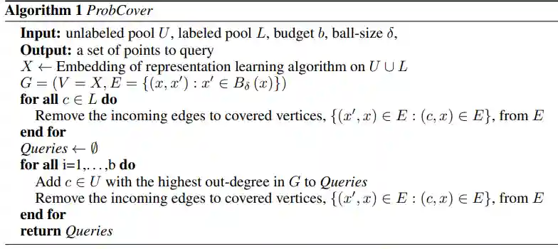
ProbCover
From my understanding, ProbCover tells you how to sample the points that have the maximum coverage for a certain space, independently of the model that you will use. This is motivated by the observation that if we fix the of the ball covers that we would like to use, then the upper bound of the probability of the error is fixed.
The simple algorithm is just maximizing the points that have most neighbors inside its circle. This has some theoretical motivations. The main results you should remember are the following:
- The probability of impure balls in the coverage is upper bounded by the probability of impure balls in the whole sample space.
- The generalization error is upper bounded by the probability of the uncovered space and the wrongly classified points inside the covered space.
- If we fix a , which is the radius of a Ball, then we just need to maximize coverage, which could be done by the following algorithm in the image, which just maximizes for most points in the ball.
References
[1] Hübotter et al. “Transductive Active Learning: Theory and Applications” arXiv preprint arXiv:2402.15898 2024