Robbins-Moro Algorithm

The Algorithm

$$ w_{n+1} = w_{n} - \alpha_{n} \Delta w_{n} $$

For example with $\alpha_{0} > \alpha_{1} > \dots > \alpha_{n} \dots$, and $\alpha_{t} = \frac{1}{t}$ they satisfy the condition (in practice we use a constant $\alpha$, but we lose the convergence guarantee by Robbins Moro). More generally, the Robbins-Moro conditions re:

1. $\sum_{n} \alpha_{n} = \infty$
2. $\sum_{n} \alpha_{n}^{2} < \infty$ Then the algorithm is guaranteed to converge to the best answer.

One nice thing about this, is that we don’t need gradients. But often we use gradient versions (stochastic gradient descent and similar), using auto-grad, see Backpropagation. But learning with gradients brings some drawbacks:

1. We have no quantification of the uncertainty.
2. We are usually overconfident in our predictions (adversarial examples, and poor generalization to domain shifts).

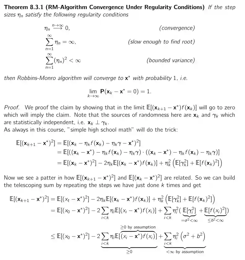
Convergence Proof

$$ \mathop{\mathbb{E}}[g(X, \theta)] = 0 $$

And $g$ is our smooth and well-behaved function.

We updated our theta iteratively based on the above rule: $\theta_{t + 1} = \theta_{t} - \alpha_{t}g(X, \theta_{t})$. Then look at this:https://chatgpt.com/share/677e4cdb-4c60-8009-b57d-49ce8efeda5a (should be verified).

Bayesian Neural Networks

The Idea

The idea here is the same as the one applied to Bayesian neural networks: define a prior of the weights and likelihood and define a posterior over the weights. But the nature of the model makes it quite difficult, if not impossible to have a closed-form solution for the posterior.

A simple model

We want to predict the weights of a given model with some bounds on certainty about them. One thing is that we have always used linear models for this, but we can also use neural networks or more complex models. Usually, in some datasets also the variance changes with the input; this is called heteroskedastic noise. This justifies models in the following form:

$$ p(y \mid \boldsymbol{x}, \theta) = \mathcal{N}(u; f_{1}(\boldsymbol{x}, \theta), \exp(f_{2}(\boldsymbol{x}, \theta))) $$

where $f_{1}$ and $f_{2}$ are neural networks and $\theta$ are the weights of the neural network. We use neural networks to predict mean and variance. We use the $\exp$ function to ensure that the variance is always positive.

From a practical point of view, this machinery is quite good at estimating variance in regions where data is present (same thing in heteroskedastic settings!), while it is overconfident in zones without data, often collapsing the variance.

Map estimate for bayesian NN 🟨–

Assume a prior $p(\theta) \sim \mathcal{N}(\theta; 0, \lambda^{-1})$ and the above parametrization of the likelihood function, let’s derive the posterior distribution, that is $p(\theta \mid y, \boldsymbol{x})$.

We notice that while in the Bayesian Linear Regression the normalization constant is disregarded, here it is dependent on the $\theta$, so we need to consider it. We can pay higher variance cost to minimize the error in the quadratic term.

$$ \hat{\theta} = \arg\min_{\theta} - \underbrace{\log p(\theta)}_{\lambda \lVert \theta \rVert ^{2}_{2}} - \sum_{i = 1}^{n} \log p(y_{i} \mid x_{i}, \theta) $$$$ \begin{align} \log p(y_{i} \mid x_{i}, \theta) &= \log \mathcal{N}(y_{i}; \mu(x_{i}, \theta), \sigma^{2}(x_{i}, \theta))) \\ & = -\frac{1}{2} \log 2\pi \sigma^{2}(x_{i}, \theta) - \frac{1}{2\sigma^{2}(x_{i}, \theta)} (y_{i} - \mu(x_{i}, \theta))^{2} \\ & = -\frac{1}{2} \log 2\pi - \frac{1}{2} \log \sigma^{2}(x_{i}, \theta) - \frac{1}{2\sigma^{2}(x_{i}, \theta)} (y_{i} - \mu(x_{i}, \theta))^{2} \\ &= \underbrace{-\frac{1}{2} \log 2\pi}_{\text{const}} -\frac{1}{2}\left[ \log \sigma^{2}(x_{i}, \theta) + \frac{ (y_{i} - \mu(x_{i}, \theta))^{2} }{\sigma^{2}(x_{i}, \theta)}\right] \end{align} $$

Here you observe that the likelihood is maximized by having high variance (plus penalty) or having correct estimates. Then adding the prior is just a regularizing term that corresponds to weight decay (a good exercise is to prove this part).

The Classification Case:

TODO: minute 22 of part 2.

Prediction with Bayesian Neural Networks

We see that prediction is just averaging over the predictions of different networks sampled from the approximate distribution that we derived from the variational inference of the weights. Some formalization could help in clearing this out.

$$ \begin{align} p(y^{} \mid x^{}, x_{1:n}, y_{1:n}) & = \int p(y^{} \mid x^{}, \theta) p(\theta \mid x_{1:n}, y_{1:n}) d\theta \ & = \mathbb{E}{\theta \sim p(\cdot \mid x{1:n}, y_{1:n})} [p(y^{} \mid x^{}, \theta)]) \ \text{Using Variational Inf.}& \approx \mathbb{E}{{\theta \sim q(\theta)}} [p(y^{} \mid x^{}, \theta)] \

\text{Monte Carlo }& \approx \frac{1}{S} \sum_{s = 1}^{S} p(y^{} \mid x^{}, \theta_{s}) \end{align} $$ The variational is usually the approximation that is introducing the most errors.

Approximating with Gaussians 🟥+

Training

Using the variational method, usually we parametrize with Gaussians. See Variational Inference. We usually use the ELBO to minimize the difference between the variational approximation and the true distribution.

$$ \log p(D) \geq \max_{q \in \mathcal{Q}} ELBO(q) = \max_{q \in \mathcal{Q}} \mathbb{E}_{q(\theta)} [\log p(D, \theta) - \log q(\theta)] $$$$ \begin{align} ELBO(q) &= \mathbb{E}_{q(\theta)} [\log p(D, \theta) - \log q(\theta)] \\ &= \mathbb{E}_{\varepsilon \sim \mathcal{N}(0, 1)} [\log p(D, \theta + \sigma \varepsilon)] - KL(q \mid p) \\ & = \mathbb{E}_{\varepsilon \sim \mathcal{N}(0, 1)} [\log p(D, \theta + \sigma \varepsilon)] - \frac{1}{2}\log \lvert \Sigma \rvert - \frac{D}{2} \log 2\pi e \end{align} $$

This is known as Bayes by backprop (2015), and is parameterized with a diagonal covariance Gaussian.
This is used to learn the covariance matrix and mean of the variational family. After, we can do inference in the following manner:

Inference

$$ \begin{align} p(y^{*} \mid x^{*}, x_{1:n}, y_{1:n})&= \int p(y^{*} \mid x^{*}, \theta) p(\theta \mid x_{1:n}, y_{1:n}) d\theta \\ &\approx \int p(y^{*} \mid x^{*}, \theta) q(\theta) d\theta \\ &\approx \frac{1}{S} \sum_{s = 1}^{S} p(y^{*} \mid x^{*}, \theta_{s}) \\ &= \frac{1}{S} \sum_{s = 1}^{S} \mathcal{N}(y^{*}; f(x^{*}, \theta_{s}), \exp(g(x^{*}, \theta_{s}))) \end{align} $$

Intuitively, variational inference in Bayesian neural networks can be interpreted as averaging the predictions of multiple neural networks drawn according to the variational posterior $q$

Unpacking uncertainties

$$ \begin{align} \text{Var}[y^{*} \mid x^{*}, x_{1:n}, y_{1:n}] &= \underbrace{\mathbb{E}_{q(\theta)}[\text{Var}[y^{*} \mid x^{*}, \theta]]}_{\text{Aleatoric}} + \underbrace{\text{Var}_{q(\theta)}[\mathbb{E}[y^{*} \mid x^{*}, \theta]] }_{\text{Epistemic}} \\ &\approx \frac{1}{m} \sum_{s = 1}^{m} \exp(g(x^{*}, \theta_{s})) + \frac{1}{m - 1} \sum_{s = 1}^{m} (\mu(x^{*}, \theta_{s}) - \bar{\mu})^{2} \end{align} $$

Where $\bar{\mu} = \frac{1}{m} \sum_{s = 1}^{m} \mu(x^{*}, \theta_{s})$.

Bayes by Backprop 🟨

This section covers the idea of one quite influential paper (Blundell et al. 2015).

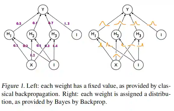
Image from the paper.This is the whole idea introduced in this document, but for historical reasons, it is due to treat it here. One of the main innovations introduced is the use of a derivative friendly method to compute an approximation for the variational lower bound principle.

In this work, they propose a generalization of the reparametrization trick, the same one used for training variational autoencoders (see Autoencoders)

$$ \frac{\partial}{\partial \theta} \mathbb{E}_{q(\mathbf{w}|\theta)}[f(\mathbf{w}, \theta)] = \mathbb{E}_{q(\epsilon)} \left[ \frac{\partial f}{\partial \mathbf{w}} \frac{\partial \mathbf{w}}{\partial \theta} + \frac{\partial f}{\partial \theta} \right]. $$$$ \frac{\partial}{\partial \mu} \mathbb{E}_{q(\mathbf{w}|\theta)}[f(\mathbf{w}, \theta)] = \mathbb{E}_{q(\epsilon)} \left[ \frac{\partial f}{\partial \mathbf{w}} 1 + \frac{\partial f}{\partial \mu} \right]. $$$$ \frac{\partial}{\partial \sigma} \mathbb{E}_{q(\mathbf{w}|\theta)}[f(\mathbf{w}, \theta)] = \mathbb{E}_{q(\epsilon)} \left[ \frac{\partial f}{\partial \mathbf{w}}\varepsilon + \frac{\partial f}{\partial sigm} \right]. $$

For the variance.

Disadvantages of Bayes by Backprop 🟨++

• Increased Computation: BBB requires sampling from the posterior distribution of weights during both training and inference, which significantly increases computational overhead compared to standard neural networks.
• Slower Convergence: The need to approximate the posterior distribution can lead to slower convergence during training.
• Gradient Estimation: The gradients of the variational lower bound (ELBO) with respect to the parameters of the variational distribution can have high variance, making optimization challenging.
• Variational Approximation: BBB relies on variational inference to approximate the true posterior distribution. This approximation can be inaccurate, especially if the chosen variational family is not flexible enough to capture the true posterior.

With Laplace Approximation

$$ \log p(\mathcal{D}, \theta) \approx \log p (\mathcal{D}, \hat{\theta}) + \frac{1}{2} (\theta - \hat{\theta})^{T} H(\theta - \hat{\theta}) $$$$ p(\mathcal{D}) = p(\mathcal{D}, \hat{\theta}) (2\pi)^{D/2} \lvert -H_{\theta} \rvert ^{-1/2} $$

The problem is often the Hessian, which could be unstable, or difficult to approximate. For this reason usually we use low-rank matrices, diagonal matrices, or other approximations.

Dropout as Variational Inference

Dropout and dropconnect can be seen as a special case of variational inference. It can been seen as if we are working with a probability distribution of different networks, which can be recalled as a special case of the one we have discussed above.

The Variational Family 🟨–

$$ q(\theta \mid \lambda) = \prod_{j} q_{j}(\theta_{j} \mid \lambda_{j}) $$

Where $q_{j}(\theta \mid \lambda)) = p\delta_{0}(\theta_{j}) + (1 - p) \delta_{\lambda_{j}}(\theta_{j})$ a mixture of Dirac deltas: with a certain probability $1- p$ we keep the weight, or set it to zero. Optimizing the network with dropout can be seen as optimizing the ELBO with respect of this variational family.

Inference with Dropout 🟩

One thing is using dropout during prediction to obtain uncertainty estimates. This is called Monte Carlo Dropout. The idea is very simple: keep the dropout during inference and sample from the network multiple times. The average of the predictions is the final prediction, and the variance is the uncertainty estimate.

Deep Ensembles

The Idea

We train $m$ different models from a bootstrapped dataset and then just average their prediction. This is the main idea of doing Ensembles.

We can also extend the probabilistic case to classification. In this case we just add a noise in the softmax layer to have some variability.

Inference

With this method we train different models on different data (maybe bootstrapped data, see Cross Validation and Model Selection). Then we just average the predictions of the different models. This is a very simple way to obtain uncertainty estimates, which allows to approximate the bayesian inference method.

$$ \begin{align} p(y^{*} \mid x^{*}, x_{1:n}, y_{1:n}) &= \int p(y^{*} \mid x^{*}, \theta) p(\theta \mid x_{1:n}, y_{1:n}) d\theta \\ &= \mathop{\mathbb{E}}_{\theta \sim p(\cdot \mid x_{1:n}, y_{1:n})} [p(y^{*} \mid x^{*}, \theta)] \\ &\approx \frac{1}{m} \sum_{s = 1}^{m} p(y^{*} \mid x^{*}, \theta_{s}) \end{align} $$

Markov Chain Monte Carlo

The MCMC idea

We would like here to sample from the posterior distribution of the weights using MCMC (somewhat similar to the SGLD method), and then use the samples to make predictions. This is a very general method, but it’s computationally expensive.

These methods explained in Monte Carlo Methods are exactly the same here, you can use these to sample from the posterior and then use the same tricks in #Inference (remember the Ergodic theorem) and #Unpacking uncertainties.

Often methods like SGLD or SG-HMC are used as they use stochastic gradients of a loss function, which can be obtained using automatic differentiation.

The key idea is just to sample $m$ values of the parameters and then use those values to make predictions.

Key Challenges 🟥++

There are two main challenges with these methods:

1. Storing the weights (usually to expensive).
   1. One way to circumvent this problem is to keep some snapshots or keeping some running averages (see next section).
   2. One idea is subsampling: we store some intermediate weights or predictions and use those for the final inference.
2. Burn in period is too costly.

Running averages

$$ \mu \leftarrow \frac{1}{T + 1} (T \mu + \theta) $$$$ \sigma^{2} \leftarrow \frac{1}{T + 1} (T \sigma^{2} + \theta^{T}\theta) $$

Outlook: Other methods

Stein Variational Gradient Descent

$$ \theta_{i} \leftarrow \theta_{i} + \frac{\epsilon}{n} \sum_{j = 1}^{n} k(\theta_{i}, \theta_{j}) (\nabla_{\theta_{j}} \log p(\theta_{j} \mid \mathcal{D}) - \nabla_{\theta_{j}}k(\theta_{j}, \theta_{i})) $$

I have no idea why we use this update rule, but it should be minimizing a certain divergence between the two distributions. TODO: understand this part.

Calibration

What is Calibration? 🟩

Well calibrated models have a similar accuracy to the confidence of their predictions. This is a very important property for many applications, especially in medical fields. For example, if a model is well calibrated, if it is secure on a prediction, it can leave the burden from the doctors, who would just manually check the hard ones.

Expected Calibration Error 🟩–

$$ \mathbb{E}_{p \sim \hat{P}} [\lvert \mathbb{P}(\hat{Y} = Y \mid \hat{P} = p) - p \rvert ] = 0 $$$$ \mathbb{P}(\hat{Y} = y \mid \hat{P} = p) = p $$$$ \text{acc}(b) = \frac{1}{N_{b}} \sum_{i \in b} \mathbb{I}(\hat{Y}_{i} = Y_{i}) $$$$ \text{conf}(b) = \frac{1}{N_{b}} \sum_{i \in b} \hat{P}_{i} $$$$ \text{ECE} = \sum_{b = 1}^{m} \frac{N_{b}}{N} \lvert \text{acc}(b) - \text{conf}(b) \rvert $$$$ \text{MCE} = \max_{b} \lvert \text{acc}(b) - \text{conf}(b) \rvert $$

Reliability Diagrams 🟩

We group the predictions of the model into bins based on their confidence. Then we plot the average confidence score against the accuracy of the model in that bin. If the model is well calibrated, this plot should be a diagonal line.

Techniques for improving calibration

Temperature Scaling

There are many techniques to improve calibration. One of the most used is temperature scaling. This is just a scaling of the logits of the model.

Platt Scaling

Another technique is Platt scaling. This is a logistic regression on the model’s output logits, interpretable as confidence scores.

References

[1] Blundell et al. “Weight Uncertainty in Neural Networks” 2015

[2] Maddox et al. “A Simple Baseline for Bayesian Uncertainty in Deep Learning” 2019