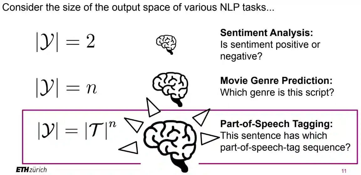
In order to understand language models we need to understand structured prediction. If you are familiar with Sentiment Analysis, where given an input text we need to classify it in a binary manner, in this case the output space usually scales in an exponential manner. The output has some structure, for example it could be a tree, it could be a set of words etc… This usually needs an intersection between statistics and computer science.

Image that summarizes the space of a structured prediction task
Definition of a language model
A language model is defined as a distribution over a $\Sigma^{*}$ (See Descrizione linguaggio for the Kleene star and the alphabet). So it assigns probabilities to $y \in \Sigma^{*}$. Remember: every element in $\Sigma^{*}$ is finite. This is important.
But we need to be careful about some details. As $\Sigma^{*}$ is an infinite set it’s not trivial to define a probability distribution over it. This motivates us to have two other definitions
Globally normalized language models
We define a scoring function $\Sigma^{*} \to \mathbb{R}$ and the normalize it over all $y \in \Sigma^{*}$. We define a scoring function $s$. Then we can do the following:
$$ p(y) := \frac{\exp(-s(y))}{\sum_{y' \in \Sigma^{*}} \exp(- s(y'))} := \frac{1}{Z} \exp(- s(y)) $$The $Z$ is a sum over an infinite set, which is often difficult to compute. Sometimes it is computable instead, the negative is for historical purposes: more similar to physics models Other problem is that the normalizer sometimes doesn’t converge. These are also sometimes called energy based LMs.
Locally normalized language models
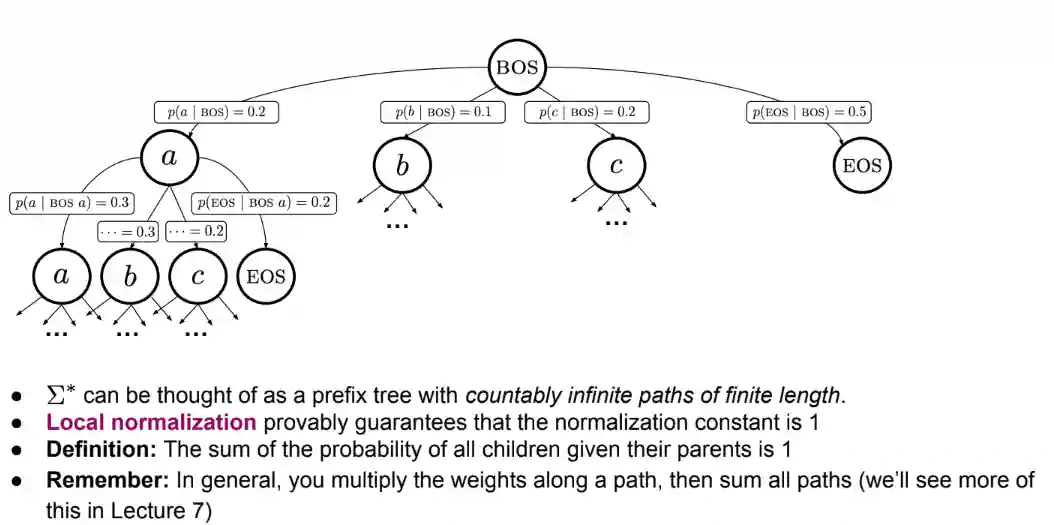
In this case, we try to take advantage of the structure of the strings, which is just a concatenation of the elements in an alphabet. Another advantage is not calculating the hideous partition function. We need a $EOS$ token and $BOS$ token in this case. Those are needed to model the starting symbol and the end symbol. Locally normalized language models model the conditional distribution $p(y \mid \boldsymbol{y})$ which means given a string $\boldsymbol{y} \in \Sigma^{*}$ try to predict $y \in \Sigma$.
$$ p(\boldsymbol{y}) = p(y_{1} \mid BOS) p(y_{2} \mid BOS y_{1}) \dots p(y_{n} \mid \boldsymbol{y}_{ In many cases where we have a structured prediction we can do something similar as the tree above.
Let’s consider a now a particular case: suppose a path in the prefix tree doesn’t have a EOS token. Then we have that sometimes the language model produces a infinite sequence of token. We say that we have deficient distributions, this is not a probability distribution anymore.
Tightness of language models
With a tight locally normalized language model we have the sum of probability of every path sums to 1. With non-tight it is possible that we lose some probability to infinite structures. It is possible to impose tightness: just set $p(EOS \mid \text{ parent}) > \varepsilon > 0$ for some $\varepsilon$.
It’s very easy to find applications for conditional language modelling, some examples are:
- In machine translation, is source-language text, and is the target-language text
- In speech recognition, is an audio signal, and is target-language text
- In summarization, is a longer text, and is a shorter text
- In dialogue systems, is a user’s input and is the agent’s response
In modern systems the following three models are the most famous ones for defining Language Models: n-gram models, recurrent neural networks and Transformers.
N-gram models
The n-gram assumption
The main idea for n-gram language models is to limit the length of the context: in this case it is not infinite but $n - 1$, meaning we only see the previous $n - 1$ tokens and not everything. Intuitively, words that are distant do not influence the current word as much as a closer. A clear drawback concerns the cases where presence of long distant relationships is important, but this is not so common.
$$ p(y_{t} \mid \boldsymbol{y}_{It’s very easy to make n-gram language models tight, we just need the probability of $EOS$ for every history to be $> 0$.
$$ \text{Number of contexes } =\sum_{j = 0}^{n - 1}\lvert \Sigma \rvert ^{j} $$Depending on the number of BOS tokens at the start. This is a quite high number of models!
Some observations
With the n-gram assumption, if we consider 1-grams they behave very much like bag of words, they just assign probability to single words, regardless of the order where they appear. Other problems with n-grams are with sparsity of the data: if a n-gram never appears, its probability is 0, which is too hard as a requirement for language modelling.
A naive implementation
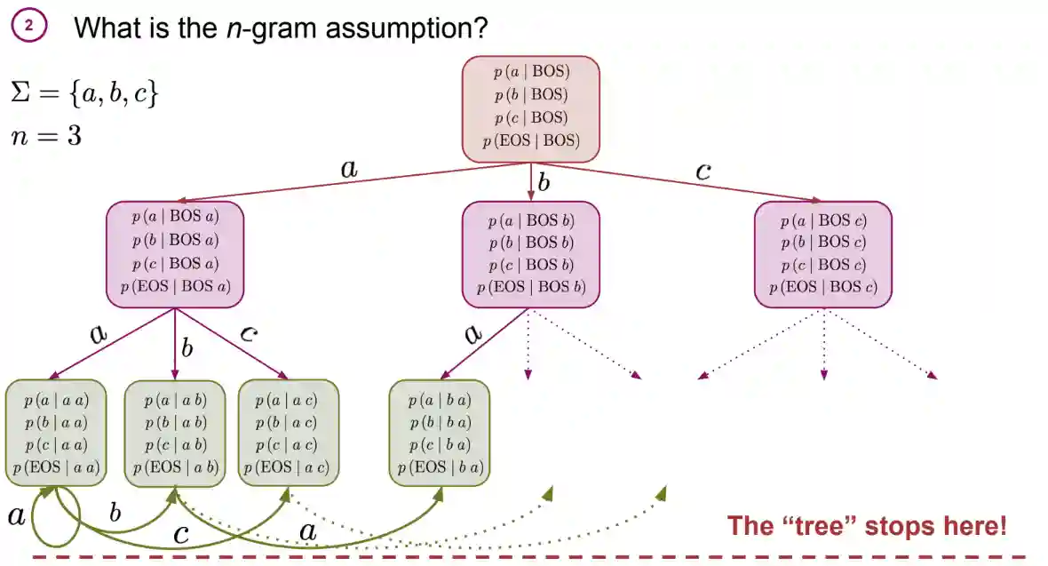
A simple solution is just define a different probability distribution for every possible context of size $n - 1$. But you can observe that this explodes exponentially: we have $\lvert \Sigma \rvert ^{n - 1}$ distributions if we assume full padding.
Number of contexes
$$ CTS = \lvert \Sigma \rvert ^{n - 1} + \lvert \Sigma \rvert ^{n - 2} \dots \lvert \Sigma \rvert + 1 = \sum_{i = 0}^{n - 1} \lvert \Sigma\rvert ^{i} $$And the number of parameters for every conditional distribution is in the size of the alphabet we want to produce, so it is $\lvert \Sigma \rvert \cdot CTS$ which is a lot if $n$ is big. This makes feasible only 2 or 3 grams.
A representation of the naive tree
Here we can clearly observe the exponential growth of the weighted prefix tree:

The Neural n-gram language
We have observed how the naive implementation explodes exponentially. This makes that model often impractical and motivates the researcher to look for more efficient methods to estimate the conditional distribution used to model the language. This model was from a Paper in 2001 conference, later JMLR journal version in 2003 (Bengio et al. 2003), it was the first language model that actually worked well. One simple idea that we will describe now is weight sharing
Weight sharing
The naive implementation has too many parameters. This is mainly caused by different representations of the context, which drives the number of needed parameters exponentially. An idea is to encode the context into a fixed size embedding, let’s say $h_{t} = enc(\boldsymbol{y}_{
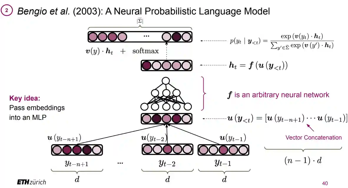
The architecture
This model was proposed in (Bengio et al. 2003) and gave state of the art performance. But is was slow. So this model is not scalable. And from the practical point of view it is almost useless. Nonetheless the ideas introduced here are of paramount historical and scientific importance.

This is the main idea
If we use an MLP with shared parameters, we can reduce the number of parameters and, hopefully, increase the ability of the model to generalize
We are using a single MLP to estimate many many conditional distributions!
Summary of the key points
As described in section 1.1 of (Bengio et al. 2003), the whole idea behind this method can be summarized in three clean points:
- Associate with each word in the vocabulary a word embedding (a real-valued vector in $\mathbb{R}^{m}$)
Which is using Word Embeddings like Mikolov’s Skip grams (at the time they probably used other kinds of embeddings, like simple Bag of words) and defining $u(\boldsymbol{y}_{
- Express the conditional probability of the next symbol in terms of the word embeddings and the output of a multilayer perceptron Using MLP to combine the embeddings producing a hidden representation $h = f(u(\boldsymbol{y}_{
- Learn the word embeddings and the parameters of the multilayer perceptron simultaneously Using Softmax to create a probability distribution $p(y_{t} \mid \boldsymbol{y}_{
- Express the conditional probability of the next symbol in terms of the word embeddings and the output of a multilayer perceptron Using MLP to combine the embeddings producing a hidden representation $h = f(u(\boldsymbol{y}_{
Many ideas present in this type of work are the same used for Transformers, this is the nice thing about science :).
NOTE: The professor in his slides presents the final softmax with a weird $v(y_{t})$ but that doesn’t seem to exist in actual implementations, where you just do everything with the concatenated embeddings. See here in tensorflow, here in pytorch. So this is a weird thing. But it’s true that the $v$ function could just return 1…
References
[1] Bengio et al. “A Neural Probabilistic Language Model” Journal of Machine Learning Research Vol. 3, pp. 1137--1155 2003