Log Linear Models can be considered the most basic model used in natural languages. The main idea is to try to model the correlations of our data, or how the posterior $p(y \mid x)$ varies, where $x$ is our single data point features and $y$ are the labels of interest. This is a form of generalization because contextualized events (x, y) with similar descriptions tend to have similar probabilities.
These kinds of models are so common that it has been discovered in many fields (and thus assuming different names): some of the most famous are Gibbs distributions, undirected graphical models, Markov Random Fields or Conditional Random Fields, exponential models, and (regularized) maximum entropy models. Special cases include logistic regression and Boltzmann machines.
Introduction to log linear models
Counting: first approach
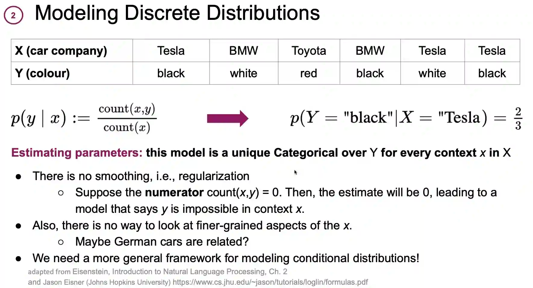
A very easy model estimating $P(y \mid x)$ is just taking the count, and assuming they are independent, so the value is $\frac{\text{count}(x, y)}{\text{ count}(x)}$. This is also the easiest model, and could have some theoretical motivations. See Naïve Bayes for example.
But it’s easy to see what problems are we getting with this simple model:

So we have two main drawbacks, described in the image.
$$ f'(x) = \begin{cases} 1 \text{, if f(x) >= 0} \\ 0 \text{ else } \end{cases} $$Exponentiation
$$ p(y \mid x) \propto \exp \text{ score } (x, y) $$$$ \exp \text{ score}(x, y) = \exp \sum_{k = 1}^{K} (\theta_{k} \cdot f_{k}(x, y)) $$We notice that the argument for the exp is always positive. At the current moment I do not understand why is this a property that we want. We would like to normalize our exponential function, so that we have a probability. We then introduce this value: $Z = \sum_{y \in Y} p(y \mid x)$. This part is usually difficult to compute, it runs in$\mathcal{O(\lvert y \rvert)}$ time.
$$ \log p(y \mid x) = \sum_{k = 1}^{K} (\theta_{k} \cdot f_{k}(x, y)) - \log Z = \vec{\theta} \cdot \vec{f}(x, y) - \log Z $$Which is a nice form. Some reasons why we are using this function is presented in the first section of The Exponential Family.
Feature pipeline
The preprocessing steps
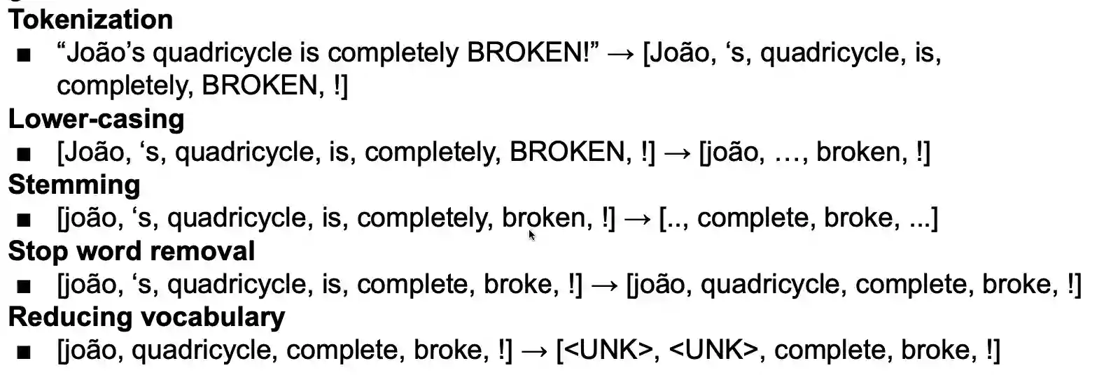
Historically, the features were hand-engineered, meaning people would try to extract functions after a step of preprocessing the text. the preprocessing step consisted in steps like
- Tokenization
- Lower casing
- stemming (getting the root of the words)
- Stop word removal
- Reducing vocabulary.
Here is an example:
 And then the input would be easy enough to be dealt with the log-linear method and the features.
Feature engineering
After we have preprocessed the texts, how can we define the features? There are some classical methods: N-grams
- (BOS, BOS, UNK), (BOS, UNK, ‘s), …, (complete, broke, ! One-hot encoding
- (0, 0, 1, 0, ..) for a single word. Bag-of-words (see spam classification)
- (0, 1, 0, 2, …), we don’t care about the order of the words, just if they are present or not in the text. Word embeddings
- Convert words into continuous representations
- Can be contextual (e.g., ELMo, BERT) or not (e.g., Glove, fastText)
- More on this in future lectures! Bag-of-embeddings
- Average embeddings for all words in a sequence Domain-specific features (for example if we know we want to agree the gender of an adjective, this feature could be built-in!)
After we have defined this, we use MLE to minimize the loss. In the case of log linear models, it is a convex function, so we have that the local minima is also the global minima, and it’s a easy problem to solve.
With the new approach, features are designed automatically with neural networks.
Expectation matching
$$ \mathcal{L}(\theta) = \sum_{n = 1}^{N} \vec{\theta} \cdot \vec{f}(x_{n} , y_{n}) - \sum_{n = 1}^{N} \log\sum_{y' \in \mathcal{Y}} p(y' \mid x_{n} ; \vec{\theta}) $$And that $p(y \mid x) = \exp(\vec{\theta} \cdot \vec{f}(x, y))$.
$$ \frac{ \partial }{ \partial \theta_{k} } \log \sum_{y \in \mathcal{Y}} \exp(\vec{\theta} \cdot \vec{f} (x, y)) = \frac{\left( \frac{ \partial }{ \partial \theta_{k} } \sum_{y \in \mathcal{Y}} \exp(\vec{\theta} \cdot \vec{f} (x, y)) \right)}{\sum_{y \in \mathcal{Y}} \exp(\vec{\theta} \cdot \vec{f} (x, y))} = \frac{ f_{k}(x, y) \sum_{y \in \mathcal{Y}} \exp(\vec{\theta} \cdot \vec{f}(x, y))}{\sum_{y \in \mathcal{Y}} p(y \mid x) } $$$$ \sum_{i = 1}^{N}f_{k}(x_{i}, y_{i}) = \sum_{i = 1}^{N} \mathbb{E}_{y}[f_{k}(x_{i}, y)] $$This tells us how we should model our $\theta$ because modifying that, has some impact on the value of the expected feature count.
$$ \frac{ \partial \mathcal{L}(\theta) }{ \partial \theta_{k} } = \sum_{n = 1}^{N} f_{k}(x_{n}, y_{n}) - \sum_{n = 1}^{N} \sum_{y' \in \mathcal{Y}} p(y' \mid x_{n}; \theta) f_{k}(x_{n}, y') $$The first part are the counts while the second part is the normalizer contribution. At the minimum we have that the above two are equal, because the derivative is zero. This is called expectation matching. (Berger 1996).
If we have Softmax Function for the loss it’s easy to explicitly write the gradient:
$$ \frac{ \partial \log \text{ softmax}(\vec{h}, y) }{ \partial \vec{\theta} } = f(x, y) - \sum_{y \in \mathcal{Y}} \text{ softmax }(\vec{h}, y) f(x, y) $$The derivation is left as exercise.
$$ \sum_{i = 1}^{N} \text{Cov}(f(x_{i}, Y)) $$Relation with linear models
One can prove that log linear models can learn any linear model. The simple reason is that in a binary-class log-linear model the decision boundary is given by $\theta g(x)$, and falls back to a Sigmoid function, this is the same as the linear model bound!
Learning Notes
People at Johns Hopkins University have done something quite nice to learn log linear models, check it out here. There are also some formulas here
This is another resource, more math heavy, for understanding log linear models in NLP. See here.
Prediction Markets
See Market Making. One famous model: see (Hanson 2007) is exactly using the properties enlisted here. It uses the derivative to act as a probability = price used within the system.
References
[1] Hanson “LOGARITHMIC MARKETS CORING RULES FOR MODULAR COMBINATORIAL INFORMATION AGGREGATION” The Journal of Prediction Markets Vol. 1(1), pp. 3--15 2007