We have a group of mappers that work on dividing the keys for some reducers that actually work on that same group of data. The bottleneck is the assigning part: when mappers finish and need to handle the data to the reducers.

Introduction

Common input formats 🟨

You need to know well what

• Shards
• Textual input
• binary, parquet and similars
• CSV and similars

Sharding 🟩

It is a common practice to divide a big dataset into chunks (or shards), smaller parts which recomposed give the original dataset. For example, in Cloud Storage settings we often divide big files into chunks, while in Distributed file systems the system automatically divides big files into native files of maximum 10 GB size.

This has two main advantages:

1. We can use the MapReduce framework to process the chunk in a highly parallelized manner.
2. We are more robust to network communication .

MapReduce

We can process terabytes of data with thousands of nodes with this architecture.

Logical Model

General framework 🟩

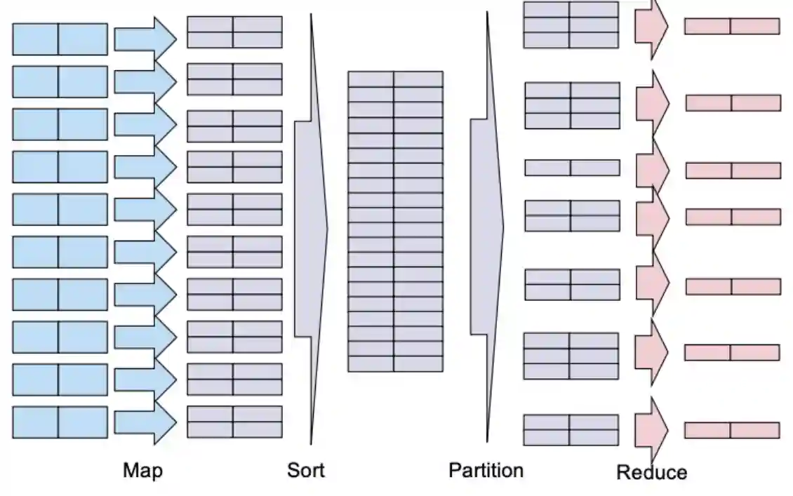We can see in the image taken from the course book [({fourny} 2024)](https://ghislainfourny.github.io/big-data-textbook/), that there are two general phases for the map reduce framework: 1. First phase is mapping, where the data is divided into chunks and processed by the mappers, then these are delivered to the designated reducers. This is usually the bottleneck, the part that runs in $\mathcal{O}(n^{2})$. 2. The reduce process connects to all other machines to get the their own mapped value. 3. Reducers then processed the partitioned, probably homogeneous data and return a result, which is often a file in HDFS.

Key Value Pairs 🟩

We have seen that MapReduce is composed of mainly two parts:

1. One part where we are extracting the data from various sources (Could be cloud, distributed files systems, wide column storages etc…)
2. We map this data to the correct reducer
   1. This part often produces some spaghetti like data flows in it. Which has some weird shapes of arrows in all directions (some parts could be more linear, while others could be more spaghetti like)
3. The final part is the reduce where the actual value is produced and stored.

The three parts in principle can have different key types, but they need to have some key type known at compile time. But often the output key and the key input to the reducer have the same type.

The Architecture

Centralized Architecture 🟩–

Hadoop MapReduce builds upon a centralized architecture compatible to Distributed file systems and HBase. In this case there is a Jobtracker, often in the same node as the NameNode; and Tasktrackers that are in the same node as the DataNodes. We have now three processes on the same machine. When MapReduce finishes, usually every TaskTracker produces a file in the disk (usually sharded, numerated increasingly). If the task fails for a node, the Jobtracker usually re-assigns the node to another.

Jobtracker’s responsibilities

The Jobtracker has many responsibilities, see (Dean & Ghemawat 2008):

• Tracking the state of each map and reduce task (idle, executed, on execution).
• Actively pinging the Tasktrackers to see if they are still active or dead.
• If a worker has died, then re-issue the task to another machine. In the case a map machine has failed, it should issue all reducers to read from the machine of the newly-assigned worker.
• Scheduling the tasks to account for locality information (meaning usually the map task needs a split that is in the same node, or on node close by it).

Impendance Mismatch 🟩

MapReduce needs to have key-values to process the files. For text, we usually use the lines and its character offset to index them. We could also use a special character to separate different parts of the text. Often this part part of preprocessing the dataset so that it is understandable by mapreduce is called impendance mismatch

Task Granularity

We subdivide the map phase into M pieces and the reduce phase into R pieces, as described above. Ideally, $M$ and $R$ should be much larger than the number of worker machines. From (Dean & Ghemawat 2008).

The reason why $M$ and $R$ should be larger is that in this manner we have better load balancing. Usual numbers are: $M$ knowing the size of the original dataset, the aim is to keep the blocks of data around 64MB, the size of a Google GFS. $R$ is usually a multiple of the number of reduce nodes. The paper reports usual numbers like: $M = 200'000$ and $R = 5'000$, using 2,000 worker machines.

Combining 🟩

This is a form of optimization. Recall that a big bottleneck of this system is the network communication, when we are mapping, we can do part of the reducing step so that later we have fewer key-value pairs to transmit. Often the combining step is the same as the reducing step. But this is not often possible:

• Type must be the same for reduce function.
• We need to have commutative and associative functions for reduce.

After the combining step we have the following diagram: 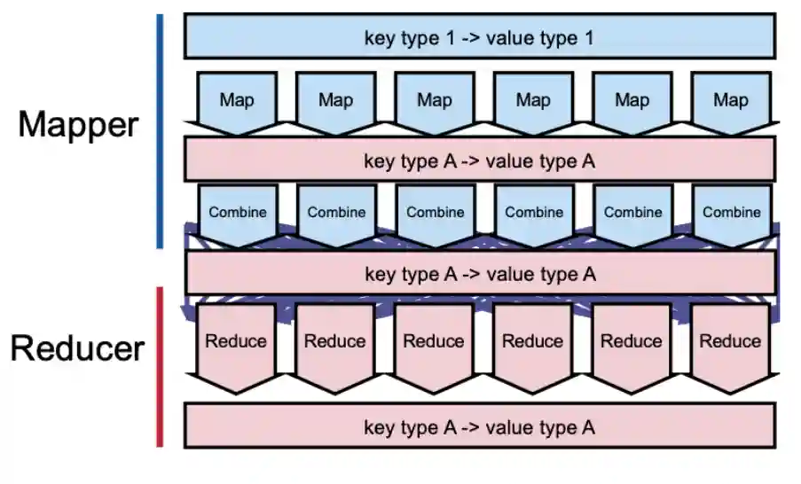And there will be less overload on the network, which makes the whole thing faster.

Rule of thumb: tasks are 3x the number of nodes that are mapping and reducing.

On Terminology

You need to know what maps, reducer and combiners are. You also need to know what tasks, slots and phases, are.

Functions 🟩

The only difference between a map and reduce function, is that the former takes a single key-value pair as input, while the second can take one or more. Both of them are functions that can produce zero, one, or more output key-value pairs. The combine function has the same definition as the reduce function.

Tasks 🟩

Tasks are sequential calls to the respective functions. If we consider map-tasks for example, then the number of map function calls within the task is the the number of key-value pairs within an input task. The input split is so divided into many mapping tasks, and each task calls the mapping function individually for each key-value pair.

Same thing could be said for reduce tasks: they are sequential calls to the reduce function on a subset of intermediate key-value pairs.

But, there are no combine tasks, as they are immediately executed after the map function, if any.

Slots 🟩

Slots are bundles of resources like CPU cores, memory resources, and network bandwidth. Usually, a single node could have more than one slot, which helps to handle the different needs for resources of different slots (some could need more memory, while others on the same node could need less memory, this better balances it).

A Map Slot is usually a single CPU core with some memory. As we have a single core, the slot processes a single map task at a time, but several map tasks after one other.

Same thing is said for Reduce Slots, but in this case we are talking about reduce functions.

Phase 🟩

The map phase is several map slots processing several map tasks in parallel. Same thing is said for the reduce phase. With the standard MapReduce framework, slots are allocated statically at the beginning, which could hinder performance. Innovation like YARN ease this problem, we will talk about this in the following sections.

Splits and Blocks 🟥

the data belonging to the split that is the input of a map task resides on the same machine as the map slot processing this map task.

Splits are map or reduce partition sets of the whole data that needs to be processed. This is physically stored in HDFS blocks. These blocks are exactly of size 128MB, which implies the first and last key-values could be splitted in different blocks. This is an inconvenience as one needs to fetch also the preceding and successive blocks. This is why in HDFS’s api one can read blocks partially. The underlying details on how these optimizations are done are not covered here.

Resource Management

We now introduce ResourceManagers, ApplicationManagers and NodeManagers. See here. For a not checked explanation.

Bottlenecks of the original version

Jobtrackers were the bottleneck and have many responsibilities.

Jobtracker’s single point of failure

With the above traditional MapReduce function, the Jobtracker is just assumed not to die: (Dean & Ghemawat 2008). This is clearly a single point of failure. Here the idea is to shift the responsibility of managing the job to some specific slot (container) within the tasktracker.

Some responsibilities of the Jobtracker

• Resource Management
• Monitoring every task’s progress
• Job scheduling

This point of failure is still not solved! The Resource Manager becomes the next point of failure within the system!

Scalability issues :🟩

This is usually a bottleneck in this model. Clusters of about 4,000 become usually very very slow and about 10,000 tasks. Another drawback is that many reducers are idle during the map phase.

Containers are virtual collections of slots (one container could have more than one map or reduce slot), each with some cpu and some amount of memory.

Other bottlenecks 🟥

1. Scalability : MapReduce has limited scalability, while YARN can scale to 10,000 nodes and 100,000 tasks, one order of magnitute higher compared to classical MapReduce!
2. Rigidity : MapReduce v1 only supports MapReduce specific jobs. There is a need, however, for scheduling non-MapReduce workloads. For instance, we would like the ability to share cluster with MPI, graph processing, and any user code.
3. Resource utilization : in MapReduce v1, the reducers wait on the mappers to finish (and vice-versa), leaving large fractions of time when either the reducers or the mappers are idle. Ideally all resources should be used at any given time.
4. Flexibility : mapper and reducer roles are decided at configuration time, and cannot be reconfigured, this is also called lack of fungibility.

Spark makes use of in-memory data too, making the access to data much faster.

Advantages of MapReduce

Nonetheless, there could be cases where MapReduce is better than Spark, for example when the data is too big to fit in memory.

• Ultra-large datasets that do not fit in memory: For massive datasets that don’t fit even across a large Spark cluster’s memory, MapReduce’s disk-based processing can be more manageable.
• Strict fault tolerance requirements: MapReduce’s fault tolerance mechanism is very robust, as it writes intermediate results to HDFS, which may be preferred in environments where data recovery is critical.
• Low hardware resources: Spark requires more memory and computational resources than MapReduce, so in resource-constrained environments, MapReduce may be a more practical choice.

ApplicationMaster and ResourceMaster

YARN decouples the scheduling of the jobs, the allocation of resource of the jobs, and the monitoring of the jobs, the first is done by the ResourceMaster, the last by the ApplicationMaster, while the middle one is done in collaboration.

This is an innovation introduced by the YARN architecture. With this new architecture we have containers and a resource manager that allocates resources to the tasks that need to be processed.

ResourceMaster

The ResourceMaster’s main job is to grant:

• leases for resources when the ApplicationManager requests it.
• Schedule the jobs, and track only the state (on queue, executed, done).
• Accept requests by clients for jobs.
• Track the resources requested by each application.

Disaster recovery

The RM recovers from its own failures by restoring its state from a persistent store on initialization. Once the recovery process is complete, it kills all the containers running in the cluster, including live ApplicationMasters. It then launches new instances of each AM. From (Vavilapalli et al. 2013).

ApplicationMaster

When a user starts a task, the resource manager elevates a container to be the application master by communicating with a process. This container then takes part of the responsibilities of the Jobtracker in the old version;

• it now tracks task state, as done with the Jobtracker,
• re-allocates other containers when one fails (expects liveliness by the worker machines)
• it asks or releases resources to the resource manager, at any time. (they are quite good with pre-emption, see Gestione delle risorse).
• Send HeartBeats to the resource-manager to signal he is still alive.

NodeManagers

These processes run on everynode in the cluster, and are responsible for:

• Monitoring the resources on the node (CPU, memory, disk, network)
• Reporting to the ResourceManager (using heartbeats)
• Managing the containers on the node. If a NodeManager dies, the ResourceManager assumes all the containers on the node are gone, and reports failure to all ApplicationManagers, who then will re-request resources and update their state tracking part.

Setting up a task 🟨

ApplicationMasters can request and release containers at any time, dynamically. A container request is typically made by the ApplicationMasters with a specific demand (e.g., “10 containers with each 2 cores and 16 GB of RAM”). If the request is granted by the ResourceManager fully or partially, this is done indirectly by signing and issuing a container token to the ApplicationMaster that acts as proof that the resource was granted. The ApplicationMaster can then connect to the allocated NodeManager and send the token. The NodeManager will then check the validity of the token and provide the memory and CPU granted by the ResourceManager. The ApplicationMaster ships the code (e.g., as a jar file) as well as parameters, which then runs as a process with exclusive use of this memory and CPU. ~From the Book ({fourny} 2024)

The main facts to keep in mind:

1. ApplicationMasters can set up and release resources dynamically at any time
2. ApplicationMasters can request resources in a fine-grained manner, asking for exactly a specific amount of resources to the ResourceManager
3. The Granting procedure uses authorization tokens.
4. Code is usually shipped by the ApplicationMaster to the worker container.
5. ApplicationMasters can be pre-empted by the ResourceManager if the resources are needed by another application.

All the information to create a container is called Container Launch Context or CLC for short. Containers usually contain many slots, in fact they can execute several tasks in parallel.

Resource tracking

Also in this case, as has been done similarly for Distributed file systems and others, we track the available resources of each machine using heartbeats sent by NodeManagers to the ResourceManager. In this way, the ResourceManager knows exacly what is the load of each node.

Scheduling methods

Queue scheduler 🟩

For example, the queue scheduler where a job takes the whole cluster one after the other. But it’s probably not efficient as it doesn’t allow for multiple-tenancy of the cluster.

Capacity Scheduler 🟩

Another way could be the hierarchical scheduler where the amount of resource is allocated a priori. This is also called capacity scheduling because the whole cluster is divided into multiple sub-clusters corresponding to a specific department in a university or parts of a company. Then, each department can use a specific local scheduler, which could be a standard fair queue.

Fair Schedule 🟨

Fair scheduling involves more complex algorithms that attempt to allocate resources in a way fair to all users of the cluster and based on the share they are normally entitled to.

It’s difficult to orchestrate the allocation of different resources. But how to allocate it correctly when the need of resources is different for other processes? Some processes could need more memory than cpu, Disk and Network Input and Output and others other resources. If some department is not using the resource, then it could be allocated to another department. There are different types of fair scheduling, the next sections briefly examine the main methods of scheduling

Steady Fair Share 🟩

This is the share of the cluster officially allocated to each department. The various departments agree upon this with each other in advance. This number is thus static and rarely changes.

Instantaneous Fair Share 🟨

this is the fair share that a department should ideally be allocated (according to economic and game theory considerations) at any point in time. This is a dynamic number that changes constantly, based on departments being idle: if a department is idle, then the instantaneous fair share of others department becomes higher than their steady fair shares.

Current Share 🟥

this is the actual share of the cluster that a department effectively uses at any point in time. This is highly dynamic. The current share does not necessarily match the instantaneous fair share because there is some inertia in the process: a department might be using more resources while another is idle. When the other department later stops being idle, these resources are not immediately withdrawn from the first department; rather, the first department will stop getting more resources, and the second department will gradually recover these resources as they get released by the first department.

Dominant Resource Fairness 🟨

The idea is quite simple: consider the dominant resource usage by each user. Then allocate the containers in a manner that is constant with respect to max resource usage ratio / number of containers. For example if Alice is using 6% of the available CPU, and Bob 3% of the available RAM, then bob should have twice as the number of containers compared to Alice.

Three types of schedule sharing

TODO: fill this in a later occasion (See page 273 of the book)

• Steady fair share:
• Instantaneous fair share:
• Current share:

References

[1] Dean & Ghemawat “MapReduce: Simplified Data Processing on Large Clusters” Communications of the ACM Vol. 51(1), pp. 107–113 2008

[2] {fourny} “The Big Data Textbook” 2024

[3] Vavilapalli et al. “Apache Hadoop YARN: Yet Another Resource Negotiator” ACM 2013