The algorithm has been the same, some ideas are in Fourier Series, but architectures change, which means there are new ways to make this algorithm even faster.
Example of transforms
We have learned in Algebra lineare numerica, Cambio di Base that linear transforms are usually a change of basis. They are matrix vector multiplications (additions and multiplications by constants). The optimizations are based on what sorts of transforms we have (e.g. Sparse Matrix Vector Multiplication, or dense versions). The same idea applies also for Fourier transforms.
Discrete Fourier Transforms
Primitive roots
It uses primitive roots of as coefficients. Discrete Fourier transform computes:
Where is the primitive root of .
The matrix is a square matrix of size and the entries are given by:
Example of DFT matrices
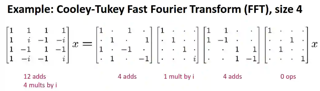
At each index we will have the th unit of root. For example if we know that the root is , then the matrix would be:
This has two adds (one add and sub), it would be quite inefficient to write the multiplication part. This is usually called butterflies in signal processing, due to the nature of the circuit.
for , the primitive root is we have:
If we assume complex everything, it has 12 additions and 4 multiplications. This matrix can be factorized, then we can add it as a series of matrix vector products.
Decomposing into sparse MVM
If , we can write:
This makes sense if are sparse (see Sparse Matrix Vector Multiplication, and not too many steps).
 You can use Group Theory to find this kind of transformations.
The above representation can be rewritten using matrix algebra:
You can see that it is also quite easy to implement it in hardware.
It can be similar for size and radix .
Other transforms
IMDCT and DCT are useful transforms for MPEG and JPEG format, while DFT and its inverse can be considered universal transformation tools.
FFT transformations
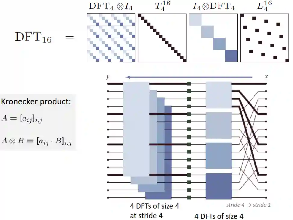
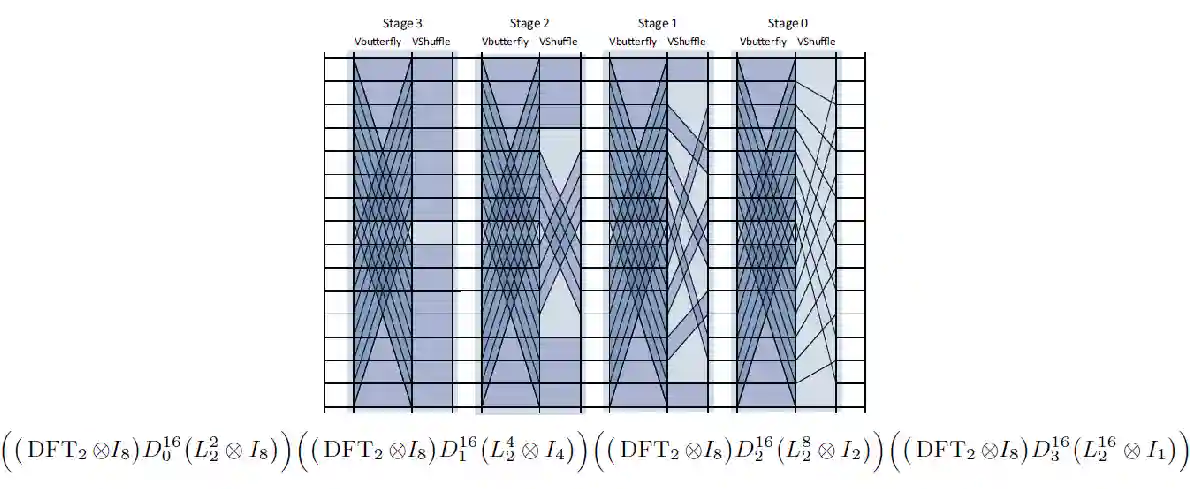
General Radix Recursive Cooley-Tukey FFT
This is the most general version of DFT, it has a similar structure compared to the previous ones.
The diagonal matrix has the roots of unity. This is called the decimation in time frequency. It is possible also to use the decimation in frequency, which is just the transpose. We can decompose everything until we have size two butterfly operations (bunch of adds).
Cost of DFT
Independently of recursion (the radix), we have a number of
- additions and multiplications, but to be real we would need to consider real additions, so we have to multiply everything by two, to get the adds. For multiplication, we have four multiplication and two additions (image it as a matrix) (in reality you use the structure of roots of unity, so in reality you have less adds). Usually best is around radix 8
- You will have about real additions and complex multiplications, so upper bound of 5 operations.
For a long time radix 2 iterative version was the best version, after superscalar processors like Skylake Microprocessor it has better versions.
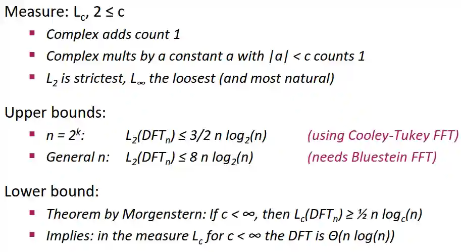 There is a practical lower bound analysis, but that is like Strassen Fast Linear Algebra, which is not much useful.
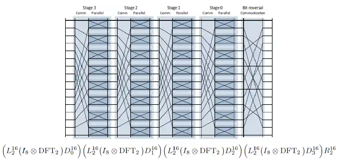
Recursive vs iterative FFT
The recursive version is good for re-use, has better locality. Triple loop is like the blocked MMM in Fast Linear Algebra. If we have big stages computed, we can continue with the next stage immediately.
Iterative similar, the op count is the same, is slower because of the (log n passes through the data). The code change is quite difficult. If we have much data, then at each iteration we need to load the whole data which could be expensive.
Decimation in Time and Frequency
TODO
Other FFTs
Pease FFT
Highly parallelized with maps and shuffles.
Stockham FFT
It is good for vector computers of the 80s, where we have long vectors
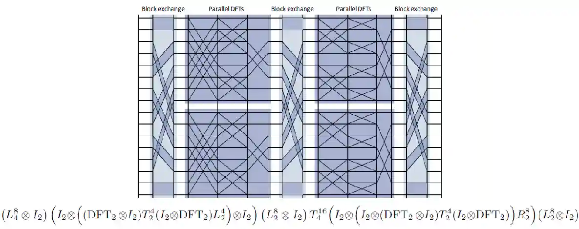
Six-Step FFT
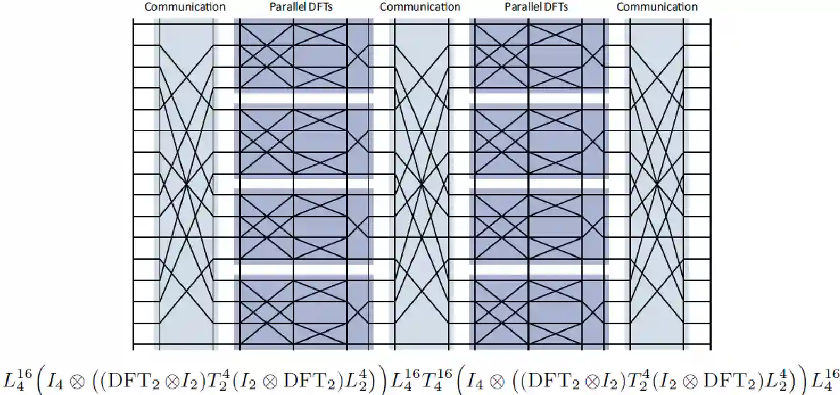
Multi-core FFT
Good for Sharing memory.
Fastest Fourier Transform of the West
Also known as FFTW, we say.
Ideas for FFTW
Merging Steps
- In the original version, the original permutation could be very expensive, to load everything. There is no need to keep it as a sperate step, we can fuse it in the next step.
- This fusion would need more data, because it needs to write to another place (no-inplace computation!).
- The scaling can also be fused, with the previous or next step (just change the kernel).
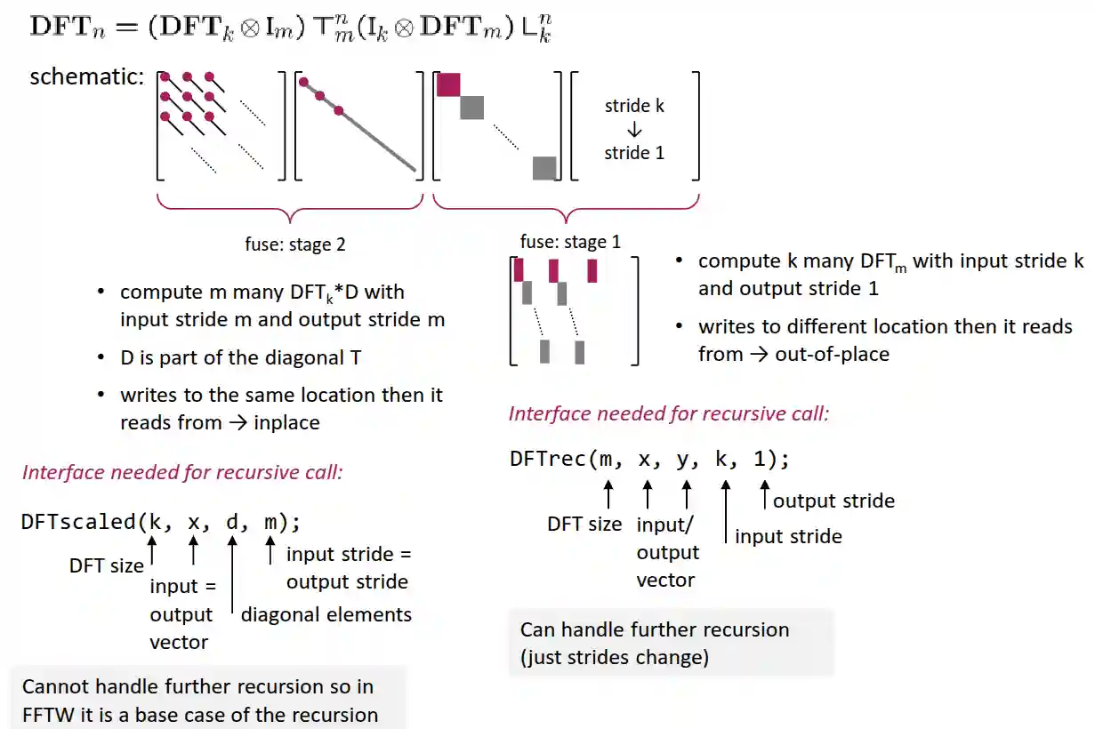
Strides will change as we recurse for the DFTrec, and we can also interchange input and output to save space. Because of the power of two strides, often it is very difficult to reach peak performance.
Constants
We precompute the constants of the sins and cosines to save time (just need what roots of unity you need in order to compute it). They just depend on the input size, so they precompute it at the beginning of the function.
Block un-rolling
We un-roll the basic blocks at the end to get longer codes, less recursion (size 32 is good basecase for example).
Program Generator
We have DAG generator (for many types of FFT), a simplifier for the DAG (specific for the FFT computation).
- An example of a simplification is when you have and , an optimization would be flipping one after you have computed one.
- Also constants come in pairs (minus and positive version).
- Reduces register pressure.