Generative Adversarial Network has been introduced in 2014 by Ian Goodfellow (at that time they where still gray and white). Now the images have been improved with Diffusion Models, that can be considered the new paradigm. This idea has been considered by Yann LeCun as one of the most important ideas. Nowadays (2025), they are still used for super-resolution and other applications, but it has still some limitations (mainly stability), and now has good competition against other models. The resolution purported by GAN is much higher than VAE (see Autoencoders#Variational Autoencoders). This is a easy plugin to improve the results of other models (VAE, flow, Diffusion). Also ChatGPT has some sort of adversarial learning for example, not explained in the same manner as here.

General Idea

Here we have two main networks that are jointly trained:

• Generator: this is a neural network that takes a random vector as input and generates a fake image. The goal of the generator is to produce images that are indistinguishable from real images.
• Discriminator: this is a neural network that takes an image as input and predicts whether it is real or fake. The goal of the discriminator is to correctly classify images as real or fake.
  • Its role is to provide some signal for the generator to create good images, it can be seen as some sort of flexible loss, intuitively.
• Adversarial Loss: the generator and discriminator are trained in an adversarial manner. The generator tries to fool the discriminator, while the discriminator tries to correctly classify images. This creates a game-like scenario where both networks improve over time. This has some sort of similarity of natural evolution when you have a predator and a prey and they co-evolve to surpass each other’s strategy.

We can define this more formally:

• Generator: $G: \mathbb{R}^{L} \to \mathbb{R}^{Q}$ where $Q \gg L$, and the discriminator is a function $D: \mathbb{R}^{Q} \to [0, 1]$.

Training a Generative Adversarial Network.

Training Process

$$ \min_{G} \max_{D} V(G,D) = \mathbb{E}_{x \sim p_{data}(x)}[\log D(x)] + \mathbb{E}_{z \sim p_{z}(z)}[\log(1 - D(G(z)))] $$

This is the original loss function, but it has some problems (like vanishing gradients). The generator tries to minimize this function, while the discriminator tries to maximize it.

Theory shows that the stable point $p_{\text{model}} = p_{\text{data}}$ but only with $G$ and $D$ have infinity capacity (they can match any data distribution, which is a quite strong assumption). In practice optimizing both jointly is quite expensive computationally. Usually you do $k$ iterations for D and $1$ for $G$ because we want to have informative output for $G$. It looks to me that this idea is quite similar to the Actor Critic model see RL Function Approximation.

With the above values, if we call $\phi$ the parameters of the discriminator and $\theta$ the parameters of the generator, we can write the optimization problem as:

$$ \begin{align*} \min_{\theta} \max_{\phi} V(\theta, \phi) &= \mathbb{E}{x \sim p{data}(x)}[\log D(x; \phi)] + \mathbb{E}{z \sim p{z}(z)}[\log(1 - D(G(z; \theta); \phi))] \ &\approx \frac{1}{N} \sum_{i=1}^{N} [\log D(x^{(i)}; \phi) + \log(1 - D(G(z^{(i)}; \theta); \phi))]

\end{align*} $$

$$ \begin{align*} \frac{\partial V(\theta, \phi)}{\partial \theta} &= \frac{1}{N} \sum_{i=1}^{N} [\frac{\partial}{\partial \theta} \log(1 - D(G(z^{(i)}; \theta); \phi))] \\ \frac{\partial V(\theta, \phi)}{\partial \phi} &= \frac{1}{N} \sum_{i=1}^{N} [\frac{\partial}{\partial \phi} \log D(x^{(i)}; \phi) + \frac{\partial}{\partial \phi} \log(1 - D(G(z^{(i)}; \theta); \phi))] \end{align*} $$

Where $x^{(i)}$ are the real samples and $z^{(i)}$ are the noise samples. And updates should also reflect minimization and maximization objectives.

$$ \begin{align*} \Delta \theta &= -\eta_{\theta} \frac{\partial V(\theta, \phi)}{\partial \theta} \\ \Delta \phi &= \eta_{\phi} \frac{\partial V(\theta, \phi)}{\partial \phi} \end{align*} $$

Problems with Likelihood

Given a generative model, we ask here, is likelihood of a certain sample a good indicator of it?

• Sometimes we have poor samples yet good likelihood, this is usually the case when you have a strong spike of likelihood values, irrelevant of the noise (e.g. $\log(0.01p(x)) = \log p(x) - \log 100$, if $p(x)$ is proportional to $d$, for independent dimensions, the first value could be very high, nonetheless having poor sample quality, this is an example from eq 11 of https://arxiv.org/pdf/1511.01844)
• Sometimes we have low likelihood yet good samples: a simple example is test data evaluation after over-fitting, models would give low likelihood to good samples, since they have not been seen during training. This means that likelihood alone is not a good metric to compare the models.

GAN Training Algorithm

It’s important to have a not too powerful and not too weak discriminator, otherwise the signal would be too strong.

While not converged do:

1. $$\nabla_{\Theta_D} \frac{1}{N} \sum_{i=1}^{N} [\log(D(x^{(i)})) + \log(1 - D(G(z^{(i)})))]$$

   * $\Theta_D$ represents the parameters of the discriminator. * $D(x)$ is the discriminator’s output for a real sample $x$ (probability that $x$ is real). * $G(z)$ is the generator’s output for a noise sample $z$ (a generated fake sample). * The goal is to maximize this objective, making the discriminator better at distinguishing real from fake samples.

2. Freeze Discriminator (D). Draw $N$ noise samples $\{z^{(1)}, ..., z^{(N)}\}$ from $p(z)$.

3. $$\nabla_{\Theta_G} \frac{1}{N} \sum_{i=1}^{N} [\log(1 - D(G(z^{(i)})))]$$
   • $\Theta_G$ represents the parameters of the generator.
   • The goal is to minimize this objective, making the generator better at fooling the discriminator into thinking its generated samples are real.

Explanation:

• The discriminator tries to learn to distinguish between real data and fake data generated by the generator.
• The generator tries to learn to produce fake data that is indistinguishable from real data, thus fooling the discriminator.

The process typically involves alternating between training the discriminator for $k$ steps and then training the generator for one step (although other ratios are possible). This ensures that the discriminator doesn’t become too strong too quickly, preventing the generator from learning useful gradients. The training continues until a convergence criterion is met, ideally when the generator produces samples that the discriminator can no longer reliably classify as fake.

Optimal behaviour requirements

$$ \mathcal{L}(D) = - \frac{1}{N} \sum_{i=1}^{N} \left[ \log D(x^{(i)}) + \log(1 - D(G(z^{(i)}))) \right] $$$$ V(G, D) = \mathop{\mathbb{E}}_{x \sim p_{\text{data}}} \left[ \log D(x) \right] + \mathop{\mathbb{E}}_{z \sim p(z)} \left[ \log(1 - D(G(z))) \right] $$

Consider $G$ is fixed, we consider here an optimal $D$.

$$ V(G, D) = \int _{x} p_{\text{data}}(x) \log (D(x)) + p_{x}(x) \log(1 - D(x)) dx $$$$ f(y) = a\log(y) + b \log(1 - y) $$$$ f'(y) = \frac{a}{a+b} $$

So the maximum of the original function is:

$$ D^{*} = \frac{p_{\text{data}}}{p_{\text{data}} + p_{x}} $$

GAN optimizes for Jensen-Shannon Divergence

To prove the following we have some strong assumptions:

• The discriminator is optimal
• The distribution of $data$ can be captured fully by $G$.

$$ D_{JS}(P \| Q) = \frac{1}{2} D_{KL}(P \| M) + \frac{1}{2} D_{KL}(Q \| M)$$

where $M = \frac{1}{2}(P + Q)$. One can prove that the min max game above is the same as optimizing for the JS divergence.

The value function of the optimal discriminator $D^*$ in a Generative Adversarial Network (GAN) is given by: $$ \begin{align*}

V(G, D^*) &= \mathbb{E}{x \sim p_d} \left[ \log \left( \frac{p_d(x)}{p_d(x) + p_m(x)} \right) \right] + \mathbb{E}{x \sim p_m} \left[ \log \left( 1 - \frac{p_d(x)}{p_d(x) + p_m(x)} \right) \right] \ & = \mathbb{E}{x \sim p_d} \left[ \log \left( \frac{p_d(x)}{p_d(x) + p_m(x)} \right) \right] + \mathbb{E}{x \sim p_m} \left[ \log \left( \frac{p_m(x)}{p_d(x) + p_m(x)} \right) \right]

\end{align*} $$ minimizing this divergence equals maximizing some likelihood.

$$ \begin{align*} V(G, D^*) &= \mathbb{E}_{x \sim p_d} \left[ \log \left( \frac{p_d(x)}{(p_d(x) + p_m(x))/2} \cdot \frac{1}{2} \right) \right] + \mathbb{E}_{x \sim p_m} \left[ \log \left( \frac{p_m(x)}{(p_d(x) + p_m(x))/2} \cdot \frac{1}{2} \right) \right] \\ &= \mathbb{E}_{x \sim p_d} \left[ \log \left( \frac{2 p_d(x)}{p_d(x) + p_m(x)} \right) - \log(2) \right] + \mathbb{E}_{x \sim p_m} \left[ \log \left( \frac{2 p_m(x)}{p_d(x) + p_m(x)} \right) - \log(2) \right] \\ &= -\log(2) + \mathbb{E}_{x \sim p_d} \left[ \log \left( \frac{2 p_d(x)}{p_d(x) + p_m(x)} \right) \right] - \log(2) + \mathbb{E}_{x \sim p_m} \left[ \log \left( \frac{2 p_m(x)}{p_d(x) + p_m(x)} \right) \right] \\ &= -2\log(2) + \int_x p_d(x) \log \left( \frac{2 p_d(x)}{p_d(x) + p_m(x)} \right) dx + \int_x p_m(x) \log \left( \frac{2 p_m(x)}{p_d(x) + p_m(x)} \right) dx \\ &= -2\log(2) + \int_x p_d(x) \log \left( \frac{p_d(x)}{(p_d(x) + p_m(x))/2} \right) dx + \int_x p_m(x) \log \left( \frac{p_m(x)}{(p_d(x) + p_m(x))/2} \right) dx \\ &= -2\log(2) + D_{KL} \left( p_d(x) \middle\| \frac{p_d(x) + p_m(x)}{2} \right) + D_{KL} \left( p_m(x) \middle\| \frac{p_d(x) + p_m(x)}{2} \right) \\ &= -2\log(2) + 2 D_{JS}(p_d(x) \| p_m(x)) \end{align*} $$

Where:

• $p_d(x)$ is the true data distribution.
• $p_m(x)$ is the distribution of the generated samples (implicitly defined by the generator $G$).
• $D^*$ is the optimal discriminator.
• $\mathbb{E}_{x \sim p}$ denotes the expectation over the distribution $p$.
• $D_{KL}(p \| q)$ is the Kullback-Leibler divergence between distributions $p$ and $q$.
• $D_{JS}(p \| q)$ is the Jensen-Shannon divergence between distributions $p$ and $q$.

Key Takeaway: The maximum value of the GAN’s discriminator loss is related to the Jensen-Shannon divergence between the real data distribution and the distribution of the generated samples. Minimizing the GAN loss (for the generator) corresponds to minimizing the Jensen-Shannon divergence between these two distributions, ideally leading $p_m(x)$ to become equal to $p_d(x)$.

Three Training Issues

• Vanishing Gradients (the same problem we have seen in Recurrent Neural Networks).
  • Using non-saturation loss.
• Model Collapse: this is a problem where the generator produces a limited variety of samples, leading to a lack of diversity in the generated images. This can happen when the generator finds a small set of images that fool the discriminator, but doesn’t explore other possibilities.
  • Unrolled GAN: they basically do less updates, more diffused iterations (unrolling parameter with gradient accumulation).
  • It is very easy to see that when the discriminator is too good, then the signal is very low for the generator to learn fast, leading to slow convergence.
    • One idea to circumvent this is to have smoother discriminator lines, so that the signal to the generator is stronger (See Mao et al 2016 or Sønderby)
    • Another is changing the signal to maximize the real image discrimination (changes the error signal by a lot!)
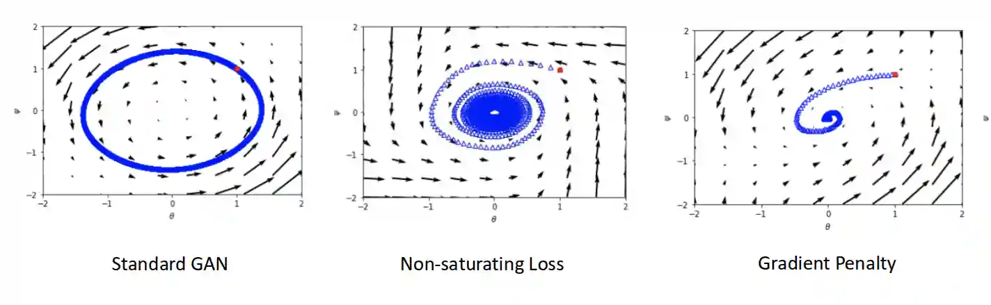
• Training Instability: GANs can be sensitive to hyperparameters, and small changes in the learning rate or architecture can lead to large changes in performance. This can make training GANs difficult and unpredictable
  • Gradient penalty: basically adding a penalty to the gradient of the discriminator’s output with respect to its input, which helps stabilize the training process. This is also known as Wasserstein GAN, since it is inspired by that distance.

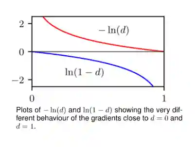
Non Saturating Loss

This loss for the GAN has been proposed by Ian Goodfellow to solve the problem in GANs. They saw that the loss for the generator was not very informative, its gradient was usually low. So the new loss for the generator is:

$$ \mathcal{L}(G, D) = -\mathbb{E}_{z}[\log D(G(z))] $$$$ \frac{\partial \mathcal{L}(G, D)}{\partial G} = - \frac{\partial D(G(z))}{\partial G} $$$$ \frac{\partial \mathcal{L}(G, D)}{\partial G} = \frac{D(G(z))}{1 - D(G(z))} \cdot \frac{\partial D(G(z))}{\partial G} $$

Not sure if the derivatives are correct, you should check this reader :). But personally I think it is better to have something that is explicitely marked as possibly wrong than nothing, for learning.

$$ \mathop{\mathbb{E}}_{z \sim p_{z}} \left[ - \log \frac{D(G(z))}{1 - D(G(z))} \right] $$

And one can prove if you have the best discriminator, this loss leads to minimize the KL divergence (see Entropy) between the real and generated distributions.

Mode Collapse

The above was a technique ok to use at the time, since the compute was limited, but now it is probably not a problem anymore. The idea was to instead of using the current discriminator’s output to train the generator, the generator is trained based on how the discriminator would respond after multiple updates. From my understanding, this technique consists in:

• Add $k$ discriminator steps, but don’t update $D$ yet.
• Compute the generator loss against the last discriminator.
• Only then update $G$ by pushing gradient in all $k$ steps of the look ahead discriminator.

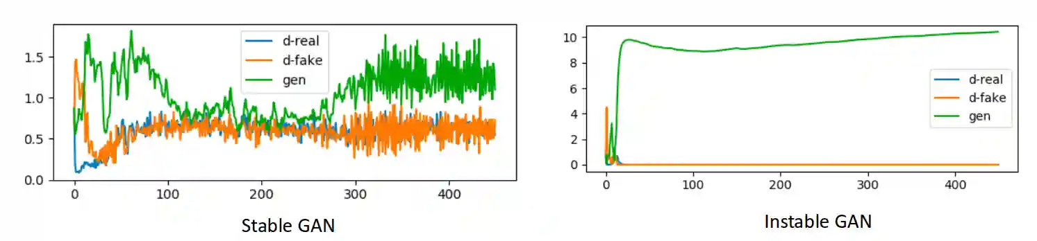
Training Instability

Since we are playing some min max game, it is very difficult to have a smooth curve. When you have a smooth curve, it is a sign that the discriminator is not good enough.

One possibility to solve this kind of problem is using gradient penalty:

$$ V(G, D) = \mathbb{E}_{x \sim p_{data}(x)}[\log D(x) ] + \mathbb{E}_{z \sim p_{z}(z)}[\log(1 - D(G(z)))] + \lambda \mathbb{E}_{x \sim p_{data}(x)}[\lVert \nabla_{x} D(x)\rVert - 1]^{2} $$

Where we want a smooth discriminator when we change the $x$ image, that loss makes the discriminator’s derivative to be closer to one, introduced in (Gulrajani et al. 2017).

This helped to created very sharp images, but there are still some problems in the images. This was built onto Wasserstein GAN (see (Arjovsky et al. 2017)).

GAN applications

High quality images can be obtained by progressively growing both the generator network and the discriminator network starting from a low resolution and then successively adding new layers that model increasingly fine details as training progresses ~(Bishop & Bishop 2024).

StyleGAN

See the paper (Karras et al. 2021): most successfullGAN model in the latest years (1K resolution generation of face images).

Stacked Training

There are two main parts for this model:

• They gradually trained stacked model from low resolution to high resolution, both generator and discriminator jointly. Down-sample the original dataset to train at that resolution, they basically started to train from small images to bigger and more complex images.

Feature modulation

• You need to be able to do feature modulation which is encoding the style and also the content to be able to generate the data. SO we need to be able to mix the content image with the style image and use this information in a correct manner.

$$ c' = \gamma(s) \odot c + \beta(s) $$

Similar to the attention mechanism.

The Architecture

They also show that they have some fine grained control on the styles by interpolating the feature functions (you can also use the features for faces, which is quite cool, and very impressive).

Image to Image translation

Pix2Pix

Introduced in Pix2Pix (Isola et al. 2018). With this problem we want to start from one kind of image, like a segmentation, and output the original image that created it, or from real image to a segmentation image, which is a cool idea.

$$ \mathcal{L}_{cyc}(G) = \mathop{\mathbb{E}}_{x,y,z} \left[ \lVert y - G(x, z) \rVert _{1} \right] $$

They have seen empirically that the L2 loss doesn’t work. Problem: You don’t always have paired images, but you need those pairs to train!

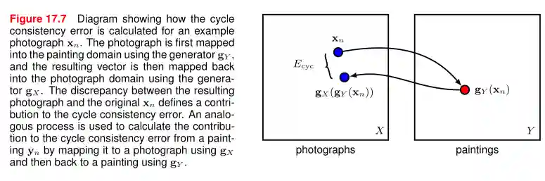
CycleGAN

We add here a L1 loss to the original loss. One drawback is that we need paired images in this case, cycleGAN solves this problem, see (Zhu et al. 2020) (guarantee that we can map back to the original image, which is another added loss), then extended to bycycleGAN (one to many, instead of one-to-one, others extended to video-to-video and autoregressive modelling).

$$ \mathcal{L}(G, F, D_{X}, D_{Y}) = \mathcal{L}_{GAN}(G, D_{Y}, X, Y) + \mathcal{L}_{GAN}(F, D_{X}, Y, X) + \lambda \mathcal{L}_{cyc}(G, F) $$$$ \mathcal{L}_{cyc}(G, F) = \mathop{\mathbb{E}}_{x,y} \left[ \lVert y - F(G(x)) \rVert _{1} + \lVert x - G(F(y)) \rVert _{1} \right] $$

The idea is that when a starting image is translated to an end image and back, they should be close to each other.

Regarding CycleGAN: Here we have pairs of generators and discriminators. Ones should generate the first kind of image, others the second kind of image, same for the generators.

Bicycle GAN

TODO

Vid2Vid

They moved from image based methods to image based videos. They extended the GAN with autoregressive models for a sequential generation.

3D-GAN

This is the same thing, just that we use 3D convolutions (and so we have voxels). But we don’t have much 3D datasets, so they used projections to 2D and classical discriminators to do the thing. This section still needs more description, TODO.

GAN for representation learning

This section mainly focuses on work done by Radford, Metz and Chintala 2015 regarding bedroom images. They have shown that following a smooth trajectory in the latent space, you can observe smooth transitions in the output space with disentangled features.

References

[1] Gulrajani et al. “Improved Training of Wasserstein GANs” Curran Associates, Inc. 2017

[2] Karras et al. “A Style-Based Generator Architecture for Generative Adversarial Networks” Vol. 43(12), pp. 4217--4228 2021

[3] Zhu et al. “Unpaired Image-to-Image Translation Using Cycle-Consistent Adversarial Networks” arXiv preprint arXiv:1703.10593 2020

[4] Bishop & Bishop “Deep Learning: Foundations and Concepts” Springer International Publishing 2024

[5] Isola et al. “Image-to-Image Translation with Conditional Adversarial Networks” arXiv preprint arXiv:1611.07004 2018

[6] Arjovsky et al. “Wasserstein Generative Adversarial Networks” PMLR 2017