Recurrent Neural Networks

Recurrent Neural Networks allows us to model arbitrarily long sequence dependencies, at least in theory (this is also why they seem a very nice choice in theory for time series). This is very handy, and has many interesting theoretical implication. But here we are also interested in the practical applicability, so we may need to analyze common architectures used to implement these models, the main limitation and drawbacks, the nice properties and some applications.

These network can bee seen as chaotic systems (non-linear dynamical systems), see Introduction to Chaos Theory.

Introduction to Recurrent Neural Networks

A simple theoretical motivation

Recall the content presented in Language Models (this is a hard prerequisite): we want an efficient way to model $p(y \mid \boldsymbol{y}_{ \lt t})$ . We have presented n-gram models (see Language Models#N-gram models) that fixate the context window thus fixating the infinite context window of a locally normalized language model, and we have developed the classical neural n-gram model. We want to build onto this and naturally invent the recurrent neural networks. Let’s start with the new content now.

We can compose the hidden state of a previous time step and the known word of the previous context in a new hidden state, and continue in this manner to produce the whole string. 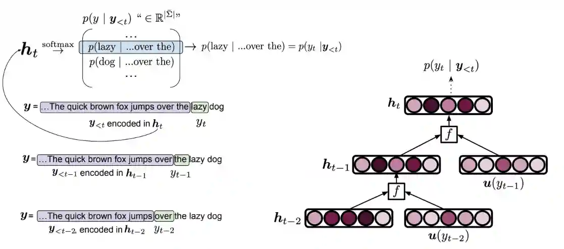This allows, in theory, to have infinite context-length. The difficult thing here is to describe $f$, that is how we combine the previous hidden state with the new token. In this context, we will call $f$ the combiner function.

Vanilla RNNs

$$ h_{t} = f(h_{t - 1}, x_{t}; \theta) $$

where we have a single function that is able to handle different kinds of inputs. We have a single hidden vector $h$.

Vanilla RNNs have the following equations:

$$ h_{t} = \tanh (W_{h} h_{t - 1} + W_{x} x_{t} + b) $$$$ o_{t} = W_{o} h_{t} + b_{o} $$

Two ways to model dynamical systems

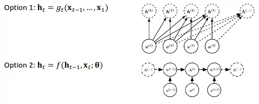RNN chose to model it with the second system, the first system is what Autoregressive Modelling does (e.g. Transformers with GPTs). You can see that the second option is much simpler.

Types of problems

Some Combiner functions

Elman Networks

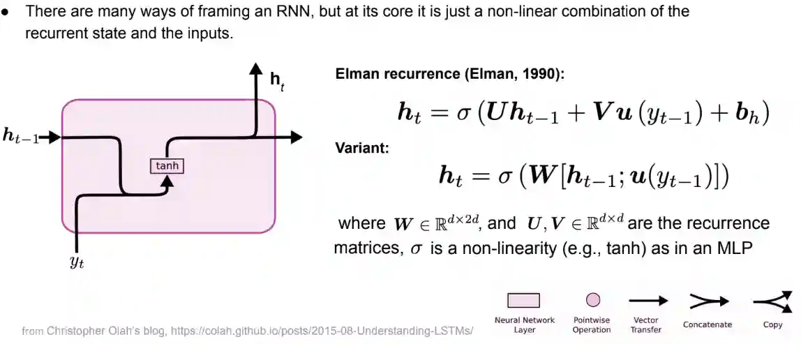This is the easiest RNN model.

LSTM Networks

The idea here is to have a leaky unit to access past information more directly, so that the gradient flows more regularly and solves that vanishing and exploding gradient problem.

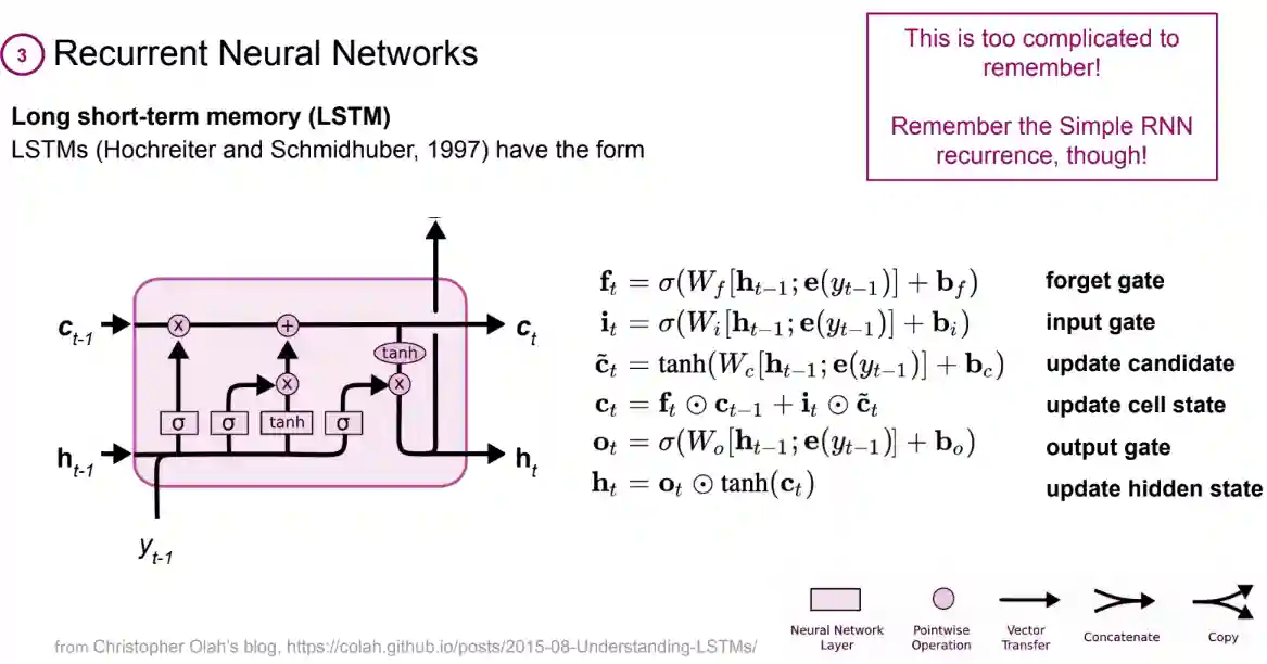
Here, you don’t need to remember the exact structure of the $f$ function, just remember that there is a way to intuitively imbue in the architecture the idea of retaining information, forgetting information and updating information. Three operations defined with weights. It’s not important to remember the architecture per se, at least if you don’t want to implement one.

• Cell state: The cell state is a vector that is maintained by the LSTM cell and is used to store information over time.
• Gates: LSTMs use three gates to control the flow of information into and out of the cell state:
  • Forget gate: The forget gate determines which information from the previous cell state to discard.
  • Input gate: The input gate determines which new information to add to the cell state.
  • Output gate: The output gate determines which information from the cell state to output.

LSTM and similar architectures solve the vanishing or exploding gradient problem by substituting them with additions.

Everything can be rewritten in a more compact manner as follows: $$ \begin{align*}

\begin{pmatrix} i_t \ f_t \ o_t \ \tilde{c}t \end{pmatrix} = \sigma \left( W \begin{pmatrix} h{t - 1} \ x_t \end{pmatrix} + b \right) \ c_t = f_t \odot c_{t - 1} + i_t \odot \tilde{c}_t \ h_t = o_t \odot \tanh(c_t) \end{align*} $$ Where $W$ is a matrix that contains all the weights of the network, and $\sigma$ is the sigmoid activation function. The $\odot$ operator denotes element-wise multiplication. NOTE: $\sigma$ at the beginning in reality should be tanh for the forget part, here it denotes activations. The LSTM architecture is designed to learn long-term dependencies in sequential data by using a combination of gates and cell states to control the flow of information.

Drawbacks of LSTM

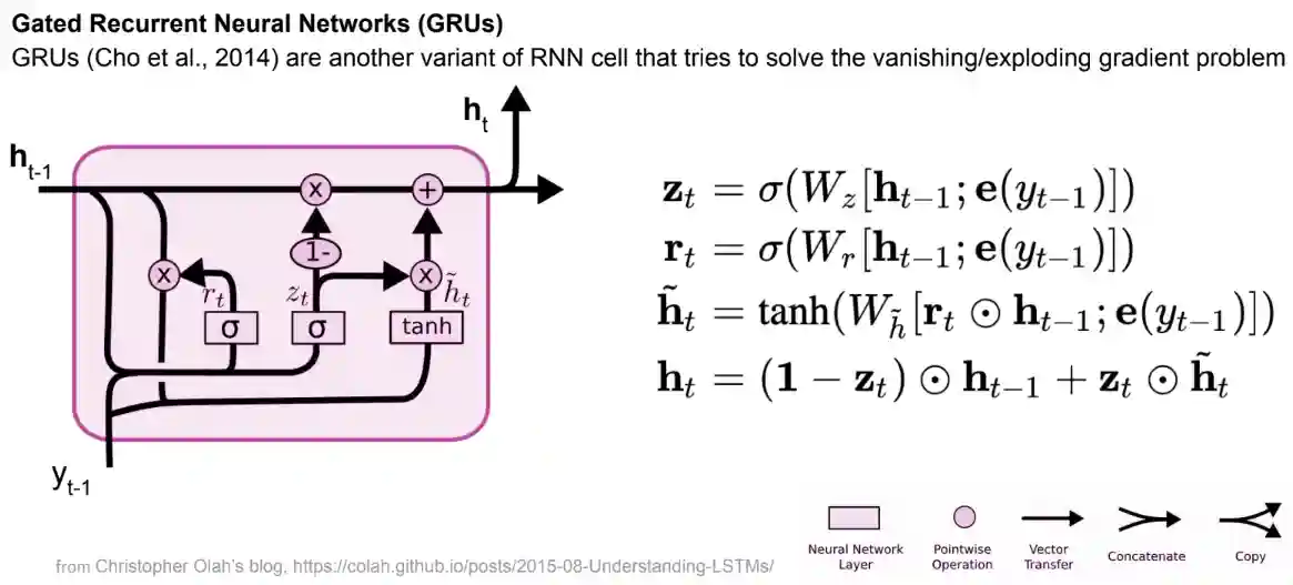
One drawback of LSTMs is that they add a lot of computation compared to RNNs, so they have developed some more lightweight versions of these networks (e.g. GRU).

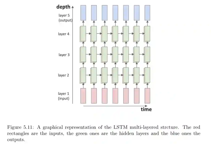
Multi Level LSTMs

GRU Networks

Stochastic RNNs

One of the bottlenecks of RNNs is their limited representation space, which is believed to constrain their generation ability.

Due to the deterministic evolution of the hidden state, RNNs model the variability in the data by means of the conditional output distributions, which may be insufficient for highly structured data such as speech and images. Such data can be characterized by the correlation between the output variables (i.e., multivariate data) and strong dependencies between variables at different time-steps (i.e., long-term dependencies). There also exists a complex relationship between the underlying factors of variation and the observed data.

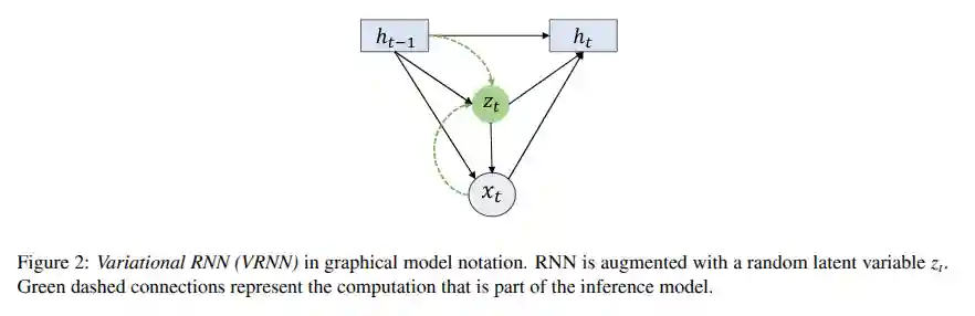
This kind of network contains a VAE at every step.

$$ h_{t } = f_{\theta}(h_{t - 1}, z_{t}, x_{t}) $$

During the recurrence step.

Formal Definitions of RNN

Real-valued Recurrent Neural Network

A deterministic real-valued recurrent neural network $\mathcal{R}$ is a four-tuple $(\Sigma, D, f, \mathbf{h}_0)$ where:

• $\Sigma$ is the alphabet of input symbols.
• $D$ is the dimension of $\mathcal{R}$.
• $f: \mathbb{R}^D \times \Sigma \rightarrow \mathbb{R}^D$ is the dynamics map, i.e., a function defining the transitions between subsequent states.
• $\mathbf{h}_0 \in \mathbb{R}^D$ is the initial state.

$$h_t = \frac{1}{2}h_{t-1} + \frac{1}{h_{t-1}}$$

This corresponds to a rational-valued RNN $(\Sigma, D, f, h_0)$ where: $\Sigma = \{a\}$ (The input alphabet consists of a single symbol ‘a’). $D = 1$ (The dimension of the RNN is 1). $f: (\mathbb{R} \times \Sigma) \rightarrow \mathbb{R}$ is given by $f(x, a) = \frac{1}{2}x + \frac{1}{x}$. * $h_0 = 2$ (The initial state is 2).

The Hidden State

The idea is to define a neural encoding function, and use that to define a language model on top of the previous definition of recurrent neural network.

Let $\mathcal{R} = (\Sigma, D, f, \mathbf{h}_0)$ be a real-valued RNN. For an input sequence $\sigma = \sigma_1 \sigma_2 \dots \sigma_T \in \Sigma^*$, the sequence of states $\mathbf{h}_0, \mathbf{h}_1, \dots, \mathbf{h}_T \in \mathbb{R}^D$ is defined inductively as follows:

• $\mathbf{h}_0$ is the initial state.
• For $1 \le t \le T$, the state at time $t$ is computed by applying the dynamics map $f$ to the previous state $\mathbf{h}_{t-1}$ and the current input symbol $\sigma_t$: $$\mathbf{h}_t = f(\mathbf{h}_{t-1}, \sigma_t)$$ The output of the RNN on the input sequence $\sigma$ is the final state $\mathbf{h}_T$.

Recurrent neural sequence model

Let $\mathcal{R} = (\Sigma, D, f, \mathbf{h}_0)$ be a recurrent neural network and $\mathbf{E} \in \mathbb{R}^{|\Sigma| \times D}$ a symbol representation matrix. A $D$-dimensional recurrent neural sequence model over an alphabet $\Sigma$ is a tuple $(\Sigma, D, f, \mathbf{E}, \mathbf{h}_0)$ defining the sequence model of the form

$$ p_{\text{SM}}(y_t \mid \mathbf{y}_{By far the most common choice of the projection function is the softmax yielding the sequence model

$$ p_{\text{SM}}(y_t \mid \mathbf{y}_{For conciseness, we will refer to RNN sequence models whose next-symbol probability distributions are computed using the softmax function as softmax RNN sequence models.

Training RNNs

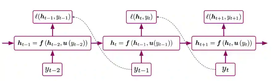
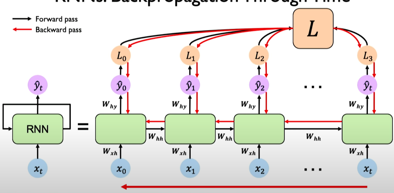
Schematic presentation of BPTT

To train RNNs we use backpropagation through time. The idea is the same as a classical Backpropagation, but we unroll the network and then use the same algorithm for backpropagation. We will update the same parameters multiple times (probably I haven’t understood this point).

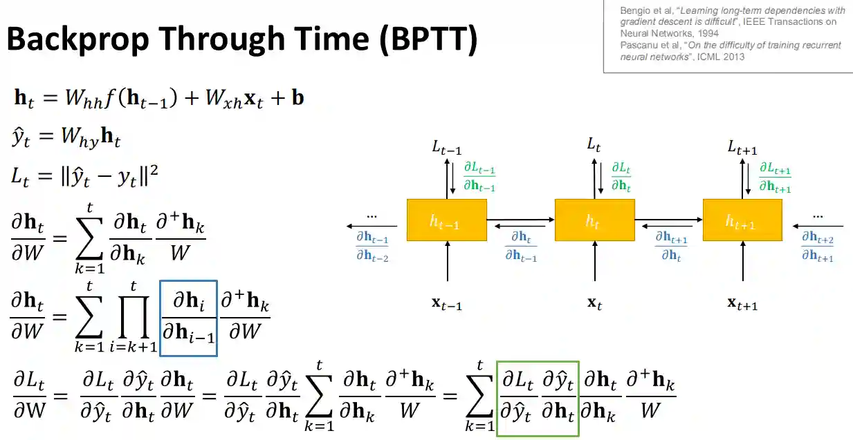
Backpropagation Through Time

• Backpropagation through time (BPTT): LSTMs use a variant of BPTT called truncated BPTT to train the network. BPTT is a technique for training recurrent neural networks by unrolling the network through time and calculating the gradients of the loss function with respect to the parameters of the network. Truncated BPTT is a simplified version of BPTT that is more computationally efficient.

It is treated as a multi-layer network with unbounded number of layers.

They are biased to more recent samples (you can observe this from the gradient information also).

Trucated BPTT

$$ \frac{ \partial h_{t} }{ \partial h_{k} } = \prod_{i = k + 1}^{t} W_{hh}^{T}\text{diag}(f'(h_{i - 1})) $$

Then we have two cases if we consider the spectral norm of the diagonal:

• If it is less than some value it is a sufficient condition that the above quantity is less than $\mu^{t - k} < 1$.
• else it is a necessary condition for it to explode, so it could happen that it does indeed explode.

This motivates to alleviate the problem by truncating the backpropagation and not going to its end.

• Vanilla RNNs are too sensitive to recent distractions.

Vanishing and Exploding gradient problem

Exploding gradients is often easy to control just with gradient clipping. The vanishing gradient problem is often more difficult to solve, we could design some:

1. Activation function
2. Weight initialization
3. Custom gate cells
4. Gradient Clipping. We will not discuss those at this moment.

It is quite easy to get an intuition of why they suffer from vanishing or exploding gradient problems. We see that $h_{t} = Wh_{t - 1}$ if W is diagonalizable then $h_{t} = Q \Lambda^{t}Q^{T} h_{1}$ and the diagonal matrix is either going to explode or going to zero since we are powering it.

Let’s do now a more formal analysis of the problem. Consider $\lambda$ to be the largest Eigenvalue of $W_{hh}$, and that the activation function is bounded by $\gamma$ (usually true, don’t use ReLU, tanh for example is a nice assumption that breaks this proof). Then it is true that $\lambda < \frac{1}{\gamma} \to$ vanishing gradient:

$$ \forall_{i} \lVert \frac{ \partial h_{i} }{ \partial h_{i - 1} } \rVert \leq \lVert W^{T}_{hh} \rVert \lVert \text{diag} \left[ f'(h_{i - 1}) \right] \rVert < \frac{1}{\gamma} \gamma = 1 $$

Then you can prove that the signal of distant $h$ is basically zero (recall the product with the h states!). When you have $\gamma > \frac{1}{\gamma}$ you have exploding gradients, but that is basically the same proof. Hochreiter and Schmidhuber say that Vanilla RNNs are too sensitive by recent distractions.

Limitations of RNN

1. Encoding the information is expected to lose something. We don’t have a clear insight about exactly what is encoded into the $h$ vectors.
2. Very slow! I can’t parallelize this computation, since one output depends on the output of the previous token!
3. In the end of the story, they can’t do long term memory at all, they say maximum is 100 words with LSTMs. Transformers solve these problems. They don’t have hidden encoding, they just do big forwards, they are parallelizable, and can encode information depending on the context size (like n-grams). But they don’t have theoretical guaranties of possible infinite context sizes…