In questa serie di appunti proviamo a descrivere tutto quello che sappiamo al meglio riguardanti gli autoencoders Blog di riferimento Blog secondario che sembra buono

Introduzione agli autoencoders

L’idea degli autoencoders è rappresentare la stessa cosa attraverso uno spazio minore, in un certo senso è la compressione con loss. Per cosa intendiamo qualunque tipologia di dato, che può spaziare fra immagini, video, testi, musica e simili. Qualunque cosa che noi possiamo rappresentare in modo digitale possiamo costruirci un autoencoder. Una volta scelta una tipologia di dato, come per gli algoritmi di compressione, valutiamo come buono il modello che riesce a comprimere in modo efficiente e decomprimere in modo fedele rispetto all’originale. Abbiamo quindi un trade-off fra spazio latente, che è lo spazio in cui sono presenti gli elementi compressi, e la qualità della ricostruzione. Possiamo infatti osservare che se spazio latente = spazio originale, loss di ricostruzione = 0 perché basta imparare l’identità. In questo senso si può dire che diventa sensato solo quando lo spazio originale sia minore di qualche fattore rispetto all’originale. Quando si ha questo, abbiamo più difficoltà di ricostruzione, e c’è una leggera perdita in questo senso.

Three desiderata

• Informative: it should be possible to reconstruct the original image.
• Disentangle: features inside the representation space should be cleanly separated.
• Robust: if the input is similar, then we would like the representation to be close (somewhat similar to the notion of continuity.
• Representativeness: if we take some points in the encoding, we would like this to have some corresponding value in the original space. (Somewhat similar to completeness)

First Ideas

This idea was from Lisker 1988. We would like the encoding and the original input space to share more information as possible: if $Z = \text{enc}(X)$ then we would like to maximize the mutual information between $Z$ and $X$, $\arg\max_{\theta} I(X ; enc_{\theta}(X))$. This is also called the Infomax principle.

The drawback is that this method does not produce disentangled neither robust representations.

$$ \frac{1}{n} \sum_{i \leq n} \mathop{\mathbb{E}}_{Z \mid x_{i}} \left[ \log p(x_{i} \mid Z) \right] $$

Autoencoders

Classical Autoencoders

Simple Linear Encoders

The simplest form of an autoencoder is a linear encoder, where the encoding function is a linear transformation and the decoding function is the transpose of the encoding function. In this simple linear case, one can prove that the optimal encoding function is the principal component analysis (PCA) of the data. See Principal Component Analysis. So if we have a simple three layer autoencoder deep neural networks, one can say it computes the PCA of the original data. The same cannot be said for multi-linear neural networks.

$$ E(w) = \sum_{i = 1}^{N} \lVert x_{i} - \hat{x}_{i} \rVert^{2} $$

Where $\hat{x} = \text{decode}(\text{encode}(x))$ In that case, the weights here are just the subspace that we are projecting to.The difference compared to PCA is that these vectors don’t need to be orthogonal with each other. People have proven that the solution for this optimization objective is exactly the same as the solution for PCA.

Deep Autoencoders

The difference compared to the previous section is that here we add some non-linear activation functions.

Such a network effectively performs a nonlinear form of PCA. It has the advantage of not being limited to linear transformations

Sparse Autoencoders

The difference compared to other methods is that here we constrain the internal representation is to use a regularizer to encourage a sparse representation, leading to a lower effective dimensionality.

$$ \tilde{E}(w) = E(w) + \lambda \sum_{k = 1}^{K} \lVert z_{k} \rVert $$

Denoising Autoencoders

In this case, we add some noise to the input and we try to reconstruct the original image. This is a way to make the network more robust to noise. So the difference compared to

Variational Autoencoders

Questi sono Autoencoders con un approccio variazionale, che abbiamo studiato in Variational Inference, ossia invochiamo in aiuto distribuzioni note e conosciute per cercare di approssimare altre distribuzioni molto più complesse, e teniamo questo come distribuzione vera da cui andiamo a prendere.

Intuizione

L’idea sembra avere uno spazio regolarizzato, ossia un $z \sim \mathcal{N}(\mu, \sigma^{2}I)$ con $\sigma$ vettore di dimensione spazio latente e $\mu$ degli offset che rappresentano media. Quindi il decoder parametrizzato secondo $\theta$ dovrà essere in una forma dipendente da questa. Questo è un prior che segue un approccio di genere generativo.

Insieme a questo utilizziamo anche un encoder parametrizzato con $\phi$ che dovrà darci indicazioni su $z$, per esempio media e varianza.

Secondo Murphy-1, Questo dovrebbe essere molto simile a un lavoro di uno 95, vedi capitolo su VAE in que libro. La formulazione dei VAE sembra molto simile ai Factor Analysis. Che è una caratterizzazione di un certo tipo sia spazio latente che quello normale.

General framework

Quello che andiamo a fare è computare una rappresentazione $p_{\theta}(z \mid x)$ dove $z$ è il nostro spazio latente con un certo prior (questo è un posterior), e poi rigenerare con un $p_{\theta'}(x \mid z)$ che è la nostra likelihood.

Setting del problema

$$ p(x | z) \sim \mathrm{N}(media, varianza) $$

Ossia i samples della parte condizionata nello spazio latente non sono altro che una media e varianza dipendenti solo dalla parte condizionale, mentre $p(z) = N(0, 1)$ multidimensionale (quindi varianza $I$)

ELBO e derivazione

Per trattare ELBO, andare a rivedersi le note in Variational Inference. Se assumiamo questo, allora la loss di Kullback-Leibler diventa abbastanza carina, perché infatti abbiamo che

$$ KL(q_{x}(z), p(z|x)) = E_{x \sim q_{x} }(\log(q_{x}(z))) - E_{x \sim q_{x}}\left(\log( \frac{p(x, z)}{p(x)}) \right)

$$ $$$$ Ora le ultime due si chiamano rispettivamente **evidence** e **ELBO** che sta per Evidence Lower Bound Notiamo che la evidence non dipende da $z$, infatti avremmo che $$

E_{z \sim q_{x}}(p(x)) = \int {-\infty}^{+\infty} q{x}(z) p(x) , dz = p(x) \int {-\infty}^{+\infty} q{x}(z) dz = p(x) $$ Quindi se vogliamo minimizzare la divergenza, ci basta Massimizzare ELBO nel nostro caso.

Esplicitazione di ELBO

Possiamo lavorare ancora di più su ELBO, provando ad esplicitarne alcuni valori, infatti possiamo considerare

$$ ELBO = E_{z \sim q_{x}}\left( \log\left( \frac{p(x, z)}{q_{x}(z)} \right) \right) =E_{z \sim q_{x}}\left( \log\left( p(x|z) \right) \right) + E_{z \sim q_{x}}\left( \log\left( \frac{p(z)}{q_{x}(z)} \right) \right) $$$$ = E_{z \sim q_{x}}\left( \log\left( p(x|z) \right) \right) - KL(q_{x}(z), p(z)) $$

Ossia abbiamo il secondo termine che prova a regolarizzare la distribuzione $q$ trovata, e il primo termine che è un maximum likelihood, simile a quanto trovato per Naïve Bayes nel corso di Asperti, che è spesso chiamato errore di ricostruzione.

Ora l’ultimo passo sarebbe come esplicitare ELBO in modo che possa essere implementato come loss di una net?

Derivazione della loss per VAE

Vedere qui, è calcolosa, ma molto carina, e ti permette di impratichirti con gaussiane multi-variabili.

Alla fine si avrà come risultato:

$$ KL(q_{x}(z), p(z)) = -\frac{1}{2} \sum_{j=1}^{J}(1 + \log \sigma^{2}_{j} - \mu^{2}_{j} - \sigma^{2}_{j}) $$

Derivazione di KL per la loss vedere Gaussians.

Per l’expectation della forma quadratica vedere qui https://statproofbook.github.io/P/mean-qf.html. Allora, sappiamo che $p(z) = \mathcal{N}(0, \mathcal{I})$ quindi ha una forma ben nota, dovremo cercare di fare questa piccolissima derivazione.

Training di VAE

Una volta ben definito la loss di ricostruzione e la loss di regolarizzazione, possiamo procedere con l’addestramento del modello allenando sia l’encoder che il decoder assieme.

Beta-VAE

Beta-VAE allows for more disentangled latent spaces.

The disentangling Idea

We want to clearly disentangle the latent dimensions of the VAE. Here we explore how individual dimensions control specific features in the output. This is useful for example introduced in (Higgins et al. 2017), going over a direction changes also identity, while we would only like to change face orientation. With this we assume we have conditionally dependent and independent factors in the latent space.

Modification of the Loss

Beta-VAE achieves the above objective by modifying the training objective of the VAE. We assume there are some conditionally independent and dependent factors in the $z$ latent variable. We use Lagrange Multipliers to model the current loss: The loss now becomes:

$$ \begin{align*} \max_{\phi, \theta}x \mathop{\mathbb{E}}_{z \sim q_{\phi}( \cdot \mid x)} \left[ \log p_{\theta}(x \mid z) \right] - \beta \cdot (KL(q_{\phi}(z \mid x) \parallel p(z)) - \delta) \\ \geq \mathop{\mathbb{E}}_{z \sim q_{\phi}( \cdot \mid x)} \left[ \log p_{\theta}(x \mid z) \right] - \beta \cdot KL(q_{\phi}(z \mid x) \parallel p(z)) \end{align*} $$

Where $\delta, \beta > 0$, this can be rewritten in some sort of ELBO, $\beta = 1$ we have the same loss of the VAE. We are basically adding a parameter to check how much is the regularization of the KL doing.

Limitations

• blurry images generation
• Probably because of the injected noise of the Gaussians
• Or weak inference models.

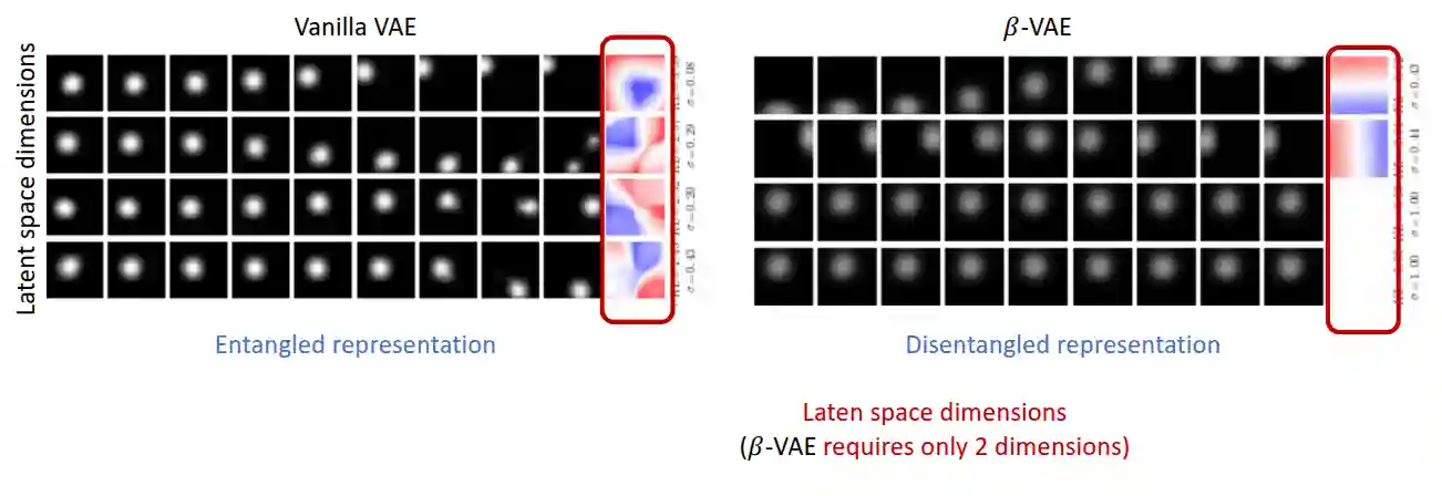They show that beta VAE effectively disentangles all the possible features correctly, while Vanilla VAE are not able to learn disentangled directions.

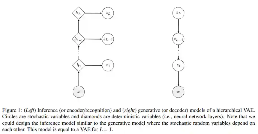
Hierarchical Latent Variable Models

$$ q_{\phi}(z_{1}, \dots, z_{L} \mid x) = \prod_{l=1}^{L} q_{\phi}(z_{l} \mid x) $$$$ p_{\theta}(z_{1}, \dots, z_{L} \mid x) = \prod_{l=1}^{L} p_{\theta}(z_{l} \mid z_{l-1}) $$

Which is quite close to some kind of autoregressive model (See Autoregressive Modelling) or n-gram model (see Language Models), and also has some similarities of how Diffusion Models are trained..

Vector Quantized Variational Autoencoders

A way to map images into discrete tokens via quantization: see (Oord et al. 2018).

In normal autoencoders you just encode the input: $E(x) = z$, while in VAE you produce a distribution $q(z|x)$. In VQ-VAE you encode the input into a discrete latent space, and then you quantize it to a finite set of values (we do similar things when we do vector search, see Optimizations for DNN#Vector Search). Meaning: You try to find the most similar vector in a embeddings database -> discrete latent representations. The codebook is learned with the autoencoder.

Intuition on VQ-VAE

VQ-VAE combines the benefits of:

• Autoencoders: for dimensionality reduction and feature learning.
• Discrete latent spaces: to better model data like text, images, or audio.
• Vector quantization: to replace the continuous latent vectors with discrete ones.
  • This enables to use Transformers in the latent space, which is a nice thing.

Architecture Components

1. Encoder: $x \rightarrow z_e(x) \in \mathbb{R}^D$ This maps the input to a continuous latent space.
2. Vector Quantizer: $z_e(x) \rightarrow z_q(x) \in \mathbb{R}^D$ This replaces the encoder output with the closest vector from a learned codebook of embeddings: $$ z_q(x) = e_k \text{ where } k = \arg\min_j \| z_e(x) - e_j \|^2 $$ So you’re snapping the encoder output to its nearest discrete prototype.
3. Decoder: $z_q(x) \rightarrow \hat{x}$ Reconstructs the input from the quantized latent.
4. Codebook / Embedding Table: $e \in \mathbb{R}^{K \times D}$ Stores $K$ learnable vectors (i.e., the “vocabulary” of your latent space).

Loss Function (Three-Part)

$$ \mathcal{L} = \underbrace{\| x - \hat{x} \|^2}_{\text{Reconstruction}} + \underbrace{\| \text{sg}[z_e(x)] - e \|^2}_{\text{Codebook Loss}} + \underbrace{\beta \| z_e(x) - \text{sg}[e] \|^2}_{\text{Commitment Loss}} $$

This is equation (3) of the paper. Where:

• Reconstruction Loss: makes the output match the input.
• Codebook Loss: moves the selected codebook entry closer to encoder output.
• Commitment Loss: encourages encoder to commit to a codebook vector.

Note: sg means “stop gradient”, i.e., the gradient is not backpropagated through this path. This is how they handle the non-differentiability of the quantization step.

Feature	VAE	VQ-VAE
Latent Space	Continuous	Discrete (via codebook)
Prior	Gaussian	Typically learned separately
Sampling	Easy via reparameterization	Uses nearest neighbor (non-differentiable)
Training	KL divergence + recon	Vector quantization + recon
Expressivity	Limited by Gaussian prior	Much richer

References

[1] Higgins et al. “Beta-VAE: Learning Basic Visual Concepts with a Constrained Variational Framework” International Conference on Learning Representations 2017

[2] Oord et al. “Neural Discrete Representation Learning” arXiv preprint arXiv:1711.00937 2018