RL Function Approximation

These algorithms are good for scaling state spaces, but not actions spaces.

The Gradient Idea

Recall Temporal difference learning and Q-Learning, two model free policy evaluation techniques explored in Tabular Reinforcement Learning.

A simple parametrization

The idea here is to parametrize the value estimation function so that similar inputs gets similar values akin to Parametric Modeling estimation we have done in the other courses. In this manner, we don't need to explicitly explore every single state in the state space.

For example, a single linear parametrization for the value function gives a quite nice interpretation of why we are introducing loss functions in this case:

Let's say $V^{\pi }(x;\theta )={\theta }_x$ and $\theta$ is a vector in the size of the state space. Then the bellman update rule, which is

$$V^{\pi }(x;{\theta }_{\text{new}})=r(x,\pi (x))+\gamma \sum _{x^{\prime }}p(x^{\prime }\mid x,\pi (x))V^{\pi }(x^{{}^{\prime }};{\theta }_{\text{old}})$$

Can bee seen as a minimization problem for the following loss:

$$\forall x,{\theta }_{new,x}=\arg \underset{{\theta }_x\in \mathbb{R}}{\min }({\theta }_x-(r(x,\pi (x))+\gamma \sum _{x^{\prime }}p(x^{\prime }\mid x,\pi (x))V^{\pi }(x^{{}^{\prime }};{\theta }_{\text{old}}))){)}^2$$

Which can be written for every single state:

$${\theta }_{new}=\arg \underset{\theta \in {\mathbb{R}}^n}{\min }{\mathbb{E}}_x(V^{\pi }(x;\theta )-(r(x,\pi (x))+\gamma \sum _{x^{\prime }}p(x^{\prime }\mid x,\pi (x))V^{\pi }(x^{{}^{\prime }};{\theta }_{\text{old}})){)}^2$$

Where $x$ is drawn from some distribution that has non zero mass for every state (so that it updates every state indefinitely).

This simple motivation example opens the door for gradient descent methods for parameter estimation! The only drawback that we will see using these methods is the enormous number of samples that we need to get a good estimate of the value function.

TD-Gradient View

Recall the update for the temporal difference was a Bootstrapped Monte Carlo estimate, which gives a biased result, but nonetheless should converge to the correct result (I think, this should be validated):

$$V^{\pi }(x)=V_{\text{old}}^{\pi }(x)+{\alpha }_t(r+\gamma V_{\text{old}}^{\pi }(x^{(i)})-V_{\text{old}}^{\pi }(x))$$

We can observe that the part that multiplies ${\alpha }_t$ can bee seen as the gradient for the following loss

$$l(\theta ;x,x^{\prime })=-\frac{1}{2}(r+\gamma V_{\text{old}}^{\pi }(x^{{}^{\prime }};\theta )-V_{\text{old}}^{\pi }(x;\theta ){)}^2$$

Where the value is parameterized by theta. It's derivative, is called the TD error, indicated with $\delta (x)$. TODO: fix the mistake for the expectation of the estimate, also expand on the fact that the gradient is 1 for the linear case, so classic TD and Q-Learning are just doing gradient descent on the linear feature vector.

One nice thing about this view, is that the gradient with respect of this loss is unbiased, due to the law of large numbers, see Central Limit Theorem and Law of Large Numbers. Sometimes gradient descent with a bootstrap estimate is called stochastic semi-gradient descent.

Q-Learning View

We can have exactly the same loss for the Q-learning update rule.

$$Q^{\pi }(x,a)=Q_{\text{old}}^{\pi }(x,a)+{\alpha }_t(r+\gamma \underset{a}{\max }{Q}_{\text{old}}^{\pi }(x^{{}^{\prime }},a)-Q_{\text{old}}^{\pi }(x,a))$$

And getting the loss, given the trajectory $(x,a,r,x^{\prime })$

$$l(\theta ;x,a,r,x^{\prime })=-\frac{1}{2}(r+\gamma \underset{a}{\max }{Q}_{\text{old}}^{\pi }(x^{{}^{\prime }},a;\theta )-Q_{\text{old}}^{\pi }(x,a;\theta ){)}^2$$

Deep Q-networks

DQN updates the neural network used for the approximate bootstrapping estimate infrequently to maintain a constant optimization target across multiple episodes.

The problem we are trying to solve is the moving optimization target property of the above q-learning optimization, which leads to instabilities (it's somewhat similar to changing the array you are iterating in, which gives unpredictable results, sometimes, or more difficult to analyze or debug).

We assume to have a dataset $\mathcal{D}$ called experience buffer. The idea here is use one network for the $old$ values, and the other used for the optimization objective. This idea is quite simple. This technique is known in the literature as Polyak averaging, or experience replay. here ${\theta }_{old}$ is not update every step, but only after $D$ iterations, which attempts to give some stability to the optimization.

$$\underset{a}{\max }q(x,a)\approx \underset{a}{\max }Q(x,a;{\theta }_{\text{old}})$$

The problem with this technique is introducing the q-value estimation, this leads to a maximization bias:

Double Q-learning

This leads to Double Q-Learning which leads to more accurate estimation of the real $q$ (Van Hasselt et al., 2016) Which is just taking the maximum with respect of the new network, and not the old. Also during gradient estimation, we are always selecting with the new network, not the old, we just use the old network to get the reward. (Meaning the $a$ inside the $Q(x,a;{\theta }_{\text{old}})$) is now taken from the new policy induced by the network parameterized with $\theta$ that changes often.

Let's quickly formalize this by viewing the loss. For standard Deep Q-learning algorithm, we have that the loss is:

$$\mathcal{L}(\theta )=\frac{1}{2}{\mathbb{E}}_{s,a,r,s^{\prime }}\left[(r+\gamma \underset{a^{\prime }}{\max }Q(s^{\prime },a^{\prime };{\theta }_{\text{old}})-Q(s,a;\theta ){)}^2\right]$$

For this modified q-learning, we use the action that maximizes the new network! Let $a^{\ast }={\max }_{a}Q(s,a;\theta )$, then the loss for double q-learning is:

$$\mathcal{L}(\theta )=\frac{1}{2}{\mathbb{E}}_{s,a,r,s^{\prime }}\left[(r+\gamma Q(s^{\prime },a^{\ast };{\theta }_{\text{old}})-Q(s,a;\theta ){)}^2\right]$$

It works quite well, but the reason why it works is not well explained mathematically. Intuitively, the old network is quite biased toward overly high values of $Q$. With Double Q-learning, we are shifting this bias towards a more accurate version, the current $Q_{\theta }$, but still evaluating using the bootstrapped old estimate.

Policy Approximation

Until now, we have always assumed to have discrete action spaces, but in other domains, we could be interested in continuous action spaces, which leads to a parameterized form of actions. So we write:

$${\pi }^{\ast }(x)=\pi (x;\phi )$$

The methods that attempt to estimate this are called policy search or policy gradient methods.

Policy Parametrization examples

For continuous spaces we might want to say that

$$\pi (a\mid x,\theta )\sim \mathcal{N}(a;\mu (x,\theta ),\Sigma (x,\theta ))$$

Where the $\mu$ and $\Sigma$ are parameterized by a Neural Network. For discrete parametrizations we might choose a classical linear network based on some features:

$$\pi (a\mid x,\theta )=Cat(a;\sigma (f(x,\theta )))$$

We can also decompose this using the Markov property if $m$ is large.

The important thing we need is:

1. Be able to use Backpropagation
2. Easy to sample from, so that we can use Monte Carlo Methods.

Function Gradient Methods

The Objective

Assume we have a policy, then we can have a rollouts for a given specific policy, which we can consider to be a sample from ${\Pi }_{\theta }(\tau )$. Then we define the function that we would like to maximize, which is

$$J_T(\theta )={\mathbb{E}}_{\tau \sim {\Pi }_{\theta }}[G_0]\approx \frac{1}{N}\sum _{i=1}^N{G}_0^{(i)}$$

Taking trajectories following the current policy.

Score Trick

We have encountered the score function before in Parametric Modeling when estimating the Rao-Cramer Bound. In this context, the score is defined as follows:

$${\nabla }_{\phi }\log {\Pi }_{\phi }=\frac{{\nabla }_{\phi }{\Pi }_{\phi }}{\Pi \phi }$$

We will use it here to get an unbiased estimate of the gradient of the policy, so that we can use Backpropagation to estimate the gradient of the policy.

The main theorem here is that the gradient we want to estimate can be rewritten as:

$${\nabla }_{\phi }{\mathbb{E}}_{\tau \sim {\prod }_{\phi }}[G_0]={\mathbb{E}}_{\tau \sim {\prod }_{\phi }}\left[G_0{\nabla }_{\phi }\log {\Pi }_{\phi }(x)\right]$$

Then we can use this estimate for the update of the gradient. Then you can also prove that in the context of the optimization of $\phi$ we can write the score as

$$\begin{array}{rl}{\nabla }_{\phi }\log {\Pi }_{\phi }(x)& ={\nabla }_{\phi }\left[\log p(x_0)+\sum _{t=0}^{T-1}\log \pi (a_t\mid x_t)+\sum _{t=0}^{T-1}\log p(x_{t+1}\mid x_t,a_t)\right]\\ & =\sum _{t=0}^{T-1}{\nabla }_{\phi }\log \pi (a_t\mid x_t)\end{array}$$

The latter is often called the eligibility vector. A common parametrization akin to Log Linear Models is the following:

$${\pi }_{\phi }(a\mid x)=\frac{\exp (h(x,a,\phi ))}{{\sum }_{a^{\prime }\in A}\exp (h(x,a^{\prime },\phi ))}$$

And $h(x,a,\phi )={\phi }^T\varphi (x,a)$ given some feature vector.

With also this trick in place, then we can take the gradient without any problems (using Monte Carlo estimation) we will then have the following:

$${\nabla }_{\phi }{J}_T(\theta )\approx \frac{1}{m}\sum _{i=1}^m{g}_{0:T}^{(i)}\sum _{t=0}^{T-1}{\nabla }_{\phi }\log \pi (a_t\mid x_t)$$

But this estimate has usually high variance.

Adding Baselines

Adding a baseline is simply choosing a constant $b$ and subtracting it to the reward estimates:

$${\mathbb{E}}_{\tau \sim {\prod }_{\phi }}\left[(G_0-b){\nabla }_{\phi }\log {\Pi }_{\phi }(x)\right]$$

Adding this constant still keeps the expectation unvaried, as the derivative of the score is 0, so it doesn't affect the estimate, but it affects the variance by reducing it if we choose $b$ correctly, which helps in the stability of the estimate.

For instance, if we choose the baseline to be

$$b_{0:t-1}=\sum _{i=0}^{t-1}{\gamma }^i{r}_i$$

Then, the adjusted gradient of the loss comes to be:

$${\nabla }_{\phi }J(\theta )\approx {\mathbb{E}}_{\tau \sim \Pi }\left[\sum _{t=0}^{T-1}{\gamma }^t{G}_{t:T}{\nabla }_{\phi }\log {\pi }_{\phi }(a_t\mid x_t)\right]$$

Which should be better in terms of its variance.

Baselines reduce variance

The condition we need to satisfy is $b^2\le 2b\cdot r(x,a)$ for each state and action. (The proof is along variance and covariance of the two functions).

We know that the expected value of the baseline is exactly $0$, this is due to the expected value of the score function being $0$, see Parametric Modeling. We then observe this:

$$\mathbb{E}[f(x)]=\mathbb{E}[f(x)-b]+\mathbb{E}[b]=\mathbb{E}[f(x)-b]$$

Furthermore, under certain conditions we have that:

Recall that $\text{Var[X + Y]}=\text{Var[X]}+\text{Var[Y]}+2\text{Cov[X, Y]}$.

So we have that:

$$\text{Var}[f(x)-b]=\text{Var}[f(x)]+\text{Var}[b]-2\text{Cov}[f(x),b]$$

Which means that if $\text{Var}[b]\le 2\text{Cov}[f(x),b]$ then the variance of the function will be reduced.

In the case of the baseline, the variance of $b$ is exactly $\mathbb{E}[b^2(\nabla \log \pi (a\mid x{)}^2]$ One can prove that given a sample trajectory, the above state dependent baseline is a valid baseline.

REINFORCE

The Reinforce algorithm allows optimization for the policy in continuous spaces but does not guarantee the convergence to the best policy possible.

One can also add the baseline as before, and it should reduce the variance, under certain cases. (for the classical state dependent baseline is easy to see that it indeed does it).

A common technique is to further reduce the variance, and only consider step-1 updates. This is somewhat akin to Stochastic Gradient Descent on policy. One can also subtract the baseline from t onwards.

Drawbacks of REINFORCE

• These methods are On-policy because we need to simulate many many roll-outs
• High variance in the gradient estimates
• The last point implied slow convergence of the method (related to the sample efficiency)
• Not guaranteed convergence

Another drawback is the difficulty of handling the exploration-exploitation trade-off. These algorithms, along with the AC methods in the next section, are fundamentally exploitative. We usually employ random exploration or epsilon-greedy methods to explore, but usually these still might converge without actually having explored the state space enough.

Policy Gradient Method

Given a trajectory (${\tau }_{t:\infty }=(x_t,a_t,r_t,x_{t+1},\dots )$) we can write the policy gradient as:

$$\begin{array}{rl}{\nabla }_{\phi }{J}_T(\phi )& =\sum _{t=0}^{\infty }{\mathbb{E}}_{t:\infty \sim {\Pi }_{\phi }}\left[{\gamma }^t{G}_t{\nabla }_{\phi }\log \pi (a_t\mid x_t)\right]\\ & =\sum _{t=0}^{\infty }{\mathbb{E}}_{x_t,a_t}\left[{\gamma }^t{Q}^{\pi }(x_t,a_t){\nabla }_{\phi }\log \pi (a_t\mid x_t)\right]\end{array}$$

Assuming we are using a baseline that starts from the $t$ time step.

Often, the above policy gradient we derived for the REINFORCE algorithm is written in terms of discounted rate occupancy measure.

The discounted rate occupancy measure tells us how probable that after a certain number of passes we will be in a certain state.

$$d_{\pi }(x)=(1-\gamma )\sum _{t=0}^{\infty }{\gamma }^{t}p(x_t=x)$$

The $1-\gamma$ factor is a normalization constant.

We can write the policy gradient as:

$${\nabla }_{\phi }{J}_T(\phi )=\frac{1}{(1-\gamma )}\cdot {\mathbb{E}}_{x\sim d_{\pi }}\left[{\mathbb{E}}_{a\sim \pi (\cdot \mid x)}[Q^{\pi }(x,a){\nabla }_{\phi }\log \pi (a\mid x)]\right]$$

This form is known as the policy gradient theorem, it will be useful to characterize the actor critic methods.

We will see that for offline methods, explored in #Offline Actor Critic, we wont need the $\log \pi$ part, as we cannot actively explore the next state from the current state.

Policy Gradient and The Exponential Family

If the policy is characterized by a distribution in the exponential family, it is easy to derive a closed form solution for the policy gradient as above. In this section we briefly discuss some gradients that are part of this family. See The Exponential Family for a discussion on distributions of this family.

Recall that if the policy is part of the exponential family we can write it as:

$$\pi (a\mid x)=h(a)\exp (a{f}_{\phi }(x)-A(f_{\phi }(x)))$$

And written in this manner the un-baselined policy gradient is:

$$\begin{array}{rl}{\nabla }_{\phi }{J}_T(\phi )& ={\mathbb{E}}_{x\sim d_{\pi }}\left[{\mathbb{E}}_{a\sim \pi (\cdot \mid x)}[Q^{\pi }(x,a){\nabla }_{\phi }\log \pi (a\mid x)]\right]\\ & ={\mathbb{E}}_{x\sim d_{\pi }}\left[{\mathbb{E}}_{a\sim \pi (\cdot \mid x)}[Q^{\pi }(x,a){\nabla }_{\phi }(a{f}_{\phi }(x)-A(f_{\phi }(x)))]\right]\\ & ={\mathbb{E}}_{x\sim d_{\pi }}\left[{\mathbb{E}}_{a\sim \pi (\cdot \mid x)}[Q^{\pi }(x,a)(f_{\phi }(x)-{\nabla }_{\phi }A(f_{\phi }(x)){\nabla }_{\phi }{f}_{\phi }(x))]\right]\end{array}$$

We just need to plug the correct values of the exponential family in.

Actor Critic Methods

Actor critic methods describe a different family of approaches that explicitly attempt to jointly improve an approximator network for the value, called critic, and a network for the policy, called actor. These methods are, as usual, divided into online and offline actor critic methods. We will analyze and present a few different methods and their properties.

Online Actor Critic

With online methods, we

A first algorithm

The main idea here is to use an approximated $Q-$value to get an approximate policy update. The main drawback is that we are doing an approximation of an approximation, so the variance of this method should be quite high. From other point of view, this is somewhat similar to the SARSA update explained in Tabular Reinforcement Learning Usually the updates here are bootstrapped too!

The notion of Advantage

This will be the base for the so called A2C algorithm, where we use the notion of Advantage to bound the variance, in a manner similar to what we have done with the baselines.

Advantage is defined as:

$$A^{\pi }(x,a)=Q^{\pi }(x,a)-V^{\pi }(x)$$

Which describes the gain in taking a specific action in a specific state compared to the average value of the state. We can prove that

$$\forall \pi ,x\underset{a}{\max }{A}^{\pi }(x,a)\ge 0$$

This is easy to see for deterministic policies, if we choose an $a$ following the policy, then it is 0, but if it could be improved then it has positive value.

Advantage Actor Critic

This method is very similar to the original Actor Critic method: instead of using the $Q$ estimate to update the critic we use the advantage This can be view as the standard Policy Gradient method with some special baseline.

Using the notion of advantage instead of the classical policy network, we get the update rule to be:

$$\phi =\phi +{\alpha }_{\phi }{\nabla }_{\phi }\log \pi (a_t\mid x_t)A^{\pi }(x_t,a_t)$$

Which is similar to the above actor-critic model, but with lesser variance if we choose the baseline equivalent correctly.

Recall that $V(x)={\mathbb{E}}_{a\sim \pi (x)}Q(x,a)$, so this is the baseline that has been chosen for this kind of Actor-Critic network. This is probably difficult to compute, and probably not stable to estimate using MonteCarlo Networks.

One thing that is usually done, is adding the parametrized value network $V(x;\theta )$ and use that one.

Trusted Region Policy Optimization

This method is a variant of the above method, but it introduces a constraint on the policy update, so that we don't update the policy too much, which can lead to instability in the optimization. For a similar reason, we use a fixed critic for multiple iterations.

The update of the policy becomes:

$${\phi }_{t+1}=\arg \underset{\phi }{\max }J(\phi )\text{ s.t. }KL({\pi }_{{\phi }_t}\parallel {\pi }_{\phi })\le \delta$$

For a fixed $\delta$ value, which defines the trust region, which is also important for the importance weights to be stable. In this case, the cost function is slightly changed, using importance sampling:

$$J(\phi )={\mathbb{E}}_{x,a\sim {\pi }_{{\phi }_t}}\left[\frac{{\pi }_{\phi }(a\mid x)}{{\pi }_{{\phi }_t}(a\mid x)}{A}^{{\pi }_{{\phi }_t}}(x,a)\right]$$

One nice thing about TRPO is that it is possible to use this algorithm in an offline fashion as long as the policy can still be trusted (i.e. it satisfies the delta constraint).

Proximal Policy Optimization

This method is a variant of the above method, but instead of using the KL divergence, we use a penalty term in the loss function to keep the policy update close to the old policy. This algorithm has also had great influence during training of language models.

One common variant uses the following objective function:

$${\phi }_{t+1}=\arg \underset{\phi }{\max }J(\phi )-\beta \cdot KL({\pi }_{{\phi }_t}\parallel {\pi }_{\phi })$$

With $\beta >0$. Other variants might work on the importance sampling.

Group Relative Policy Optimization

With this technique, we can use the same actor network for the critic (in this sense the signal is purer from the environment)

• No separate value network for the Critic,
• Sample multiple outputs from the old policy for the same question or state,
• Treat the average reward of these outputs as the baseline,
• Anything above average yields a “positive advantage,” anything below yields a “negative advantage.”

Offline Actor Critic

One clear advantage of offline learning algorithms is the possibility of re-using past data.

The Main Idea

Recall the DQN loss function:

$$\mathcal{L}(\theta )={\mathbb{E}}_{s,a,r,s^{\prime }}\left[(r+\gamma \underset{a^{\prime }}{\max }Q(s^{\prime },a^{\prime };{\theta }_{\text{old}})-Q(s,a;\theta ){)}^2\right]$$

The main problem with the standard setting is having to maximize over the set of actions, which could be very large, or even continuous.

What we do now is assume we have a "rich enough" parametrization of $Q$ and just assume that our network is learning the maximum by itself. In this way, our loss function becomes:

$$\mathcal{L}(\theta )={\mathbb{E}}_{s,a,r,s^{\prime }}\left[(r+\gamma Q(s^{\prime },{\pi }_{\phi }(s^{\prime });{\theta }_{\text{old}})-Q(s,a;\theta ){)}^2\right]$$

Where ${\pi }_{\phi }$ is the policy network. If the policy is good enough, by Bellman Optimality condition (see Markov Processes), it will naturally converge to the maximum of the $Q$ function, one problem could be the instability of this double optimization, as we are optimizing for $Q$ and $\pi$ at the same time.

In the policy update phase, instead of taking the maximum over all possible actions, we take the policy that is yielding highest returns following the rule:

$${\phi }_{t+1}=\arg \underset{\phi }{\max }{\mathbb{E}}_{s,a\sim {\pi }_{{\phi }_t}}\left[Q(s,a;{\theta }_t)\right]=\arg \underset{\phi }{\max }J(\phi )$$

Usually, instead of sampling from $\pi$, we have an offline buffer of trajectories and sample uniformly from that buffer, but nothing prevents us to sample in an online fashion. So we write:

$${\nabla }_{\phi }J(\phi )={\mathbb{E}}_{s\sim \mu }\left[Q(s,{\pi }_{\phi }(s);{\theta }_t)\right]$$

And we can get an estimate in a similar manner for the $Q$ network:

$${\nabla }_{\phi }Q(s,a;\theta )=D\phi {\pi }_{\phi }(s)\cdot {\nabla }_{a}Q(s,a;\theta ){\mid }_{a={\pi }_{\phi }(s)}$$

Note that here we are not considering the $\log \pi (a\mid x)$ to compute the gradient for the policy. My personal take is just that we don't know how to compute this value (we don't have a forward step to compute it), so we just ignore it. Here we can see a discussion on the use of $\log \pi (a\mid x)$.

Deep Deterministic Policy Gradient

Putting everything together from the section before we get the DDPG algorithm:

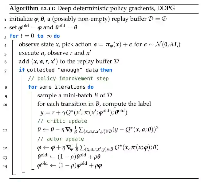
It is possible to extend this algorithm with TD3, which is a variant of the above algorithm that uses a double critic to estimate the Q-value, which helps in reducing the overestimation bias.

On Exploration

With the offline methods we have just presented, the usual solution for exploration is what is called Gaussian Noise Dithering: this method just adds some noise to the output of the policy ${\pi }_{\phi }$ in continuous settings. However, these methods often suffer from not exploring enough. The following section presents a method that attempts to ease this problem. Some methods of exploration as are also cited in Planning.

Maximum Entropy Reinforcement Learning

Maximum Entropy Reinforcement Learning (MERL) adds a regularizer that prevents the policy to become too narrow, or deterministic, for a single action. This is easily considered during the evaluation of the cost:

$$J(\phi )={\mathbb{E}}_{s,a\sim {\pi }_{\phi }}\left[Q(s,a;\theta )+\alpha \mathcal{H}({\pi }_{\phi }(\cdot \mid s))\right]$$

Where the parameter $\alpha$ is a hyper-parameter that controls how much the entropy of the policy weights.

Trust Region Policy Optimization (TRPO)

To address the instability of optimizing both $Q$ and $\pi$ simultaneously, Trust Region Policy Optimization (TRPO) introduces a constrained optimization framework. The primary idea behind TRPO is to update the policy in such a way that it stays within a trust region, ensuring that each update does not deviate excessively from the current policy. This prevents performance degradation due to overly large updates.

Objective Function: TRPO optimizes the following constrained objective:

$$\underset{\phi }{\max }{\mathbb{E}}_{s\sim \mu ,a\sim {\pi }_{{\phi }_t}}\left[\frac{{\pi }_{\phi }(a\mid s)}{{\pi }_{{\phi }_t}(a\mid s)}{A}_{{\pi }_{{\phi }_t}}(s,a)\right]$$

subject to:

$${\mathbb{E}}_{s\sim \mu }\left[D_{\text{KL}}({\pi }_{{\phi }_t}(\cdot \mid s)\parallel {\pi }_{\phi }(\cdot \mid s))\right]\le \delta ,$$

where $A_{{\pi }_{{\phi }_t}}(s,a)$ is the advantage function, $D_{\text{KL}}$ is the Kullback-Leibler divergence, and $\delta$ is a small positive constant controlling the size of the update.

Proximal Policy Optimization (PPO)

Proximal Policy Optimization (PPO) simplifies TRPO by avoiding the computational complexity of solving a constrained optimization problem. PPO achieves similar benefits by clipping the policy update directly within the objective function.

Objective Function PPO modifies the policy update by introducing a clipped surrogate objective:

$${\mathcal{L}}^{\text{PPO}}(\phi )={\mathbb{E}}_{s,a}\left[\min \left(r_t(\phi )A_{{\pi }_{{\phi }_t}}(s,a),\text{clip}(r_t(\phi ),1-ϵ,1+ϵ)A_{{\pi }_{{\phi }_t}}(s,a)\right)\right],$$

where:

$$r_t(\phi )=\frac{{\pi }_{\phi }(a\mid s)}{{\pi }_{{\phi }_t}(a\mid s)},$$

and $ϵ$ is a small hyperparameter (e.g., $ϵ=0.2$) controlling the extent of clipping.

Algorithm	Advantages	Challenges
TRPO	Stable updates, trust region enforcement	Computationally expensive, complex
PPO	Simplicity, robust performance	Sensitive to hyperparameters ($ϵ$)