Mixture of Experts
There is a gate that opens a subset of the experts, and the output is the weighted sum of the outputs of the experts. The weights are computed by a gating network.
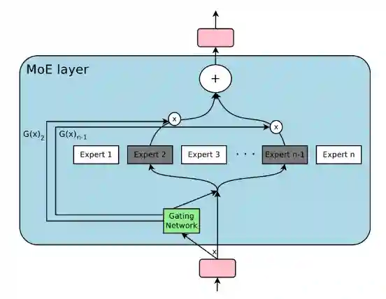
One problem is load balancing, non uniform assignment. And there is a lot of communication overhead when you place them in different devices.
LoRA: Low-Rank Adaptation
We only finetune a part of the network, called lora adapters, not the whole thing. There are two matrices here, a matrix A and B, they are some sort of an Autoencoders, done for every Q nd V matrices in the LLM attention layer. The nice thing is that there are not many inference costs if adapters are merged post training:
$$ h = Wx + BAx = (W + BA)x = W'x $$And it is very easy to switch them.
LLM Optimizations
Quadratic Bottleneck
The attention matrix scales quadratically with respect to the sequence length, which makes it difficult to store. For example, if you have a GPT2 context window of 1024 tokens, which is about 340 words, this would make your attention matrix very large with not many words.
Modern LLMs make tokens longer by having large vocabularies, and they have larger context windows (in the order of the millions for Gemini 1.5 Pro (2 Millions)).
FlashAttention
This is a systems paper which is important for computing introduced in (Dao et al. 2022). This enables exact attention computation but longer context lengths. The compute the attention matrix in a careful way to tile it inside the SRAM, this is some sort of optimization that is close to what you do in Fast Linear Algebra, they basically reduce number of memory reads and writes between GPU high bandwidth memory and on-chip SRAM (similar optimizations are done between RAM and cache, same idea basically).

Image from the paper: FlashAttention uses tiling to prevent materialization of the large $N \times N$ attention matrix (dotted box) on (relatively) slow GPU HBM.
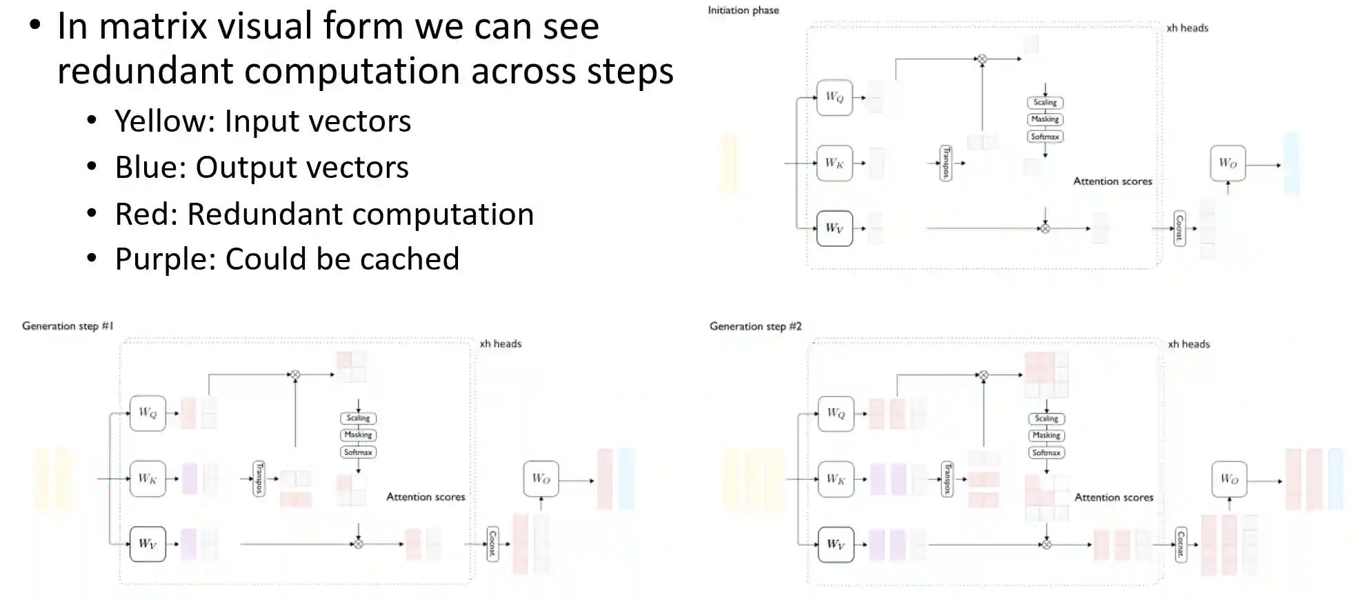
KV Caching
There is some redundant computation which is done in the attention matrix due to the autoregressive nature of the inference process. This means that instead of recomputing, we can cache some old results and not compute them again. However, this can grow a lot.
- Multiple parallel requests
- Complex decoding trategies. This was introduced in (Pope et al. 2023).
This motivates to cache Key and Values from the computation. At every step we just need to compute a single vector instead of recomputing the old values.
PagedAttention
A lot of memory of the GPU is filled by the KV Cache. PagedAttention introduces virtual pages, inspired by OS memory access in Memoria virtuale. The System assumes the KV cache is continuous, but it is actually managed in some particular manner. This brings fragmentation. Adding this virtual layer makes better use of the actual resources. The authors claim to have near zero wasted memory in the KV cache memory due to fragmentation.
Speculative Decoding
You have a small model that runs faster and attempts to predict a group of next tokens. Then you feed it to a large model and verify the tokens are correct (probable enough to have produced these tokens). This is basically Accept Reject algorithm for sampling the tokens.
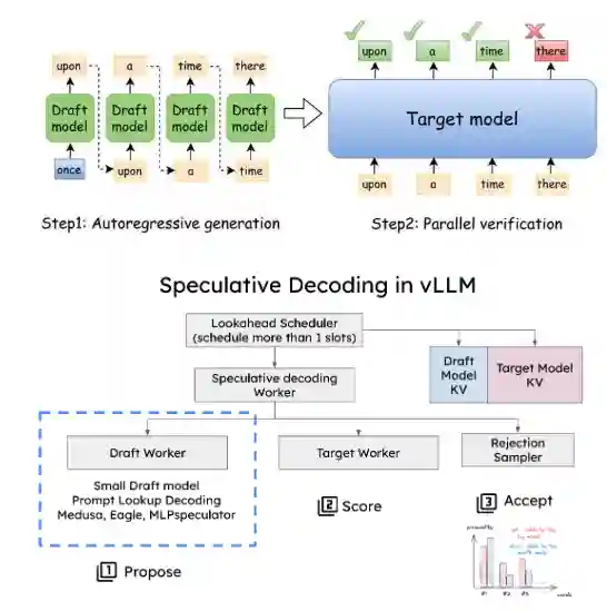 The easy example is with greedy decoding: you just accept all the tokens that match the argmax.
But LLM decoding is stochastic, so for this reason it is better to have anohter method that keeps the locality.
We use Accept Reject with acceptance probability:
The easy example is with greedy decoding: you just accept all the tokens that match the argmax.
But LLM decoding is stochastic, so for this reason it is better to have anohter method that keeps the locality.
We use Accept Reject with acceptance probability:
Where $y$ is the new token, $x$ is the prompt, $S$ is the draft fast model and $L$ is the slow model, and we assume: $L(y \mid x) \leq k \cdot S(y \mid x)$.
Batching behaviours
(He et al. 2025) is a good paper that explains most of the common optimizations that are made for LLMs. In this particular example, we have
Classical LLM serving infrastructure
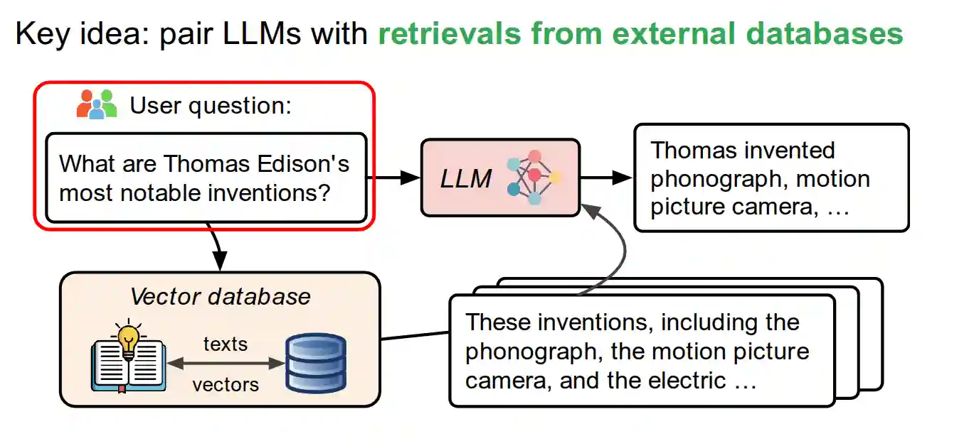
Retrieval-Augmented Generation (RAG)
Pretraining costs a lot, and updating weight knowledge using more training rounds and finetuning costs a lot. RAG addresses the problem of adding more knowledge for the model without any training, but just the so called in-context learning.
Slowly, RAG is becoming industry standard to serve LLM in a reliable manner. Prompting is becoming a normal thing.
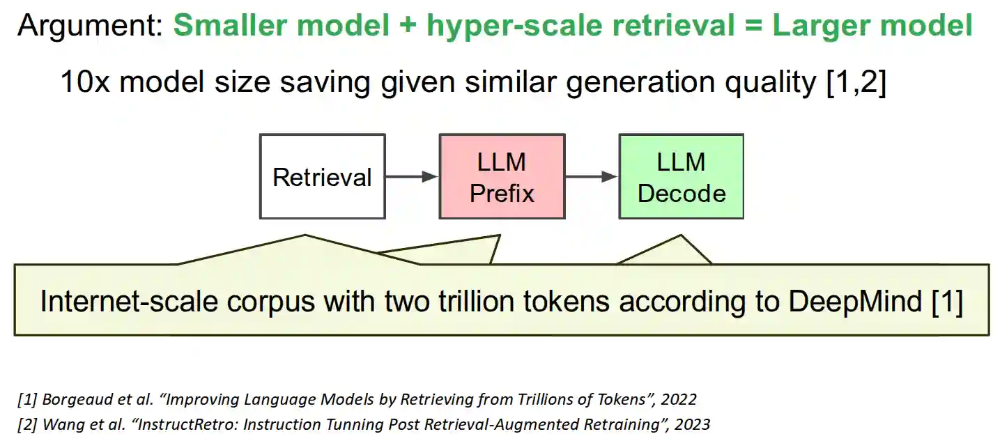
RAG with internet-scale retrieval
The pipeline is very easy: just use websearch to get many many documents, add it as a prefix to the LLM and use standard decoding.
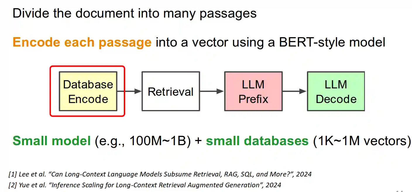
RAG for long-context processing
In many occasions, there are very very long documents that are prefixed to the LLM input. In these cases, it can be very costly to process these kinds of documents.
In this case, we just want to add relevant passages, not whole documents and use those for LLM inference. Beginning and end parts of the prompt are better processed by the model, this is a phenomenon known as lost in the middle.
RAG with iterative retrievals
In this case the model can generate a question to generate another query to retrieve other documents. This is usually used with CoT, see (Wei et al. 2023), and sequential information retrievals.
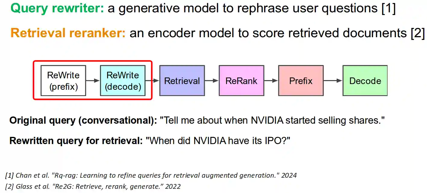
RAG with rewriter and reranker
The idea is to break down the user query into more, or rewrite the query into a format more specific for the dataset.
Vector Search
One of the classical methods are TF-IDF with document word frequency counts. The general problem is a Clustering, with nearest neighbors search.
The mathematical definition is as follows: Sure, here are the contents of the image as clean, copiable Markdown notes:
Problem statement
Given:
- A query vector $q \in \mathbb{R}^d$
- A collection of database vectors $\mathcal{D} = \{ x_1, x_2, \dots, x_N \} \subset \mathbb{R}^d$
- A similarity (or distance) function $\text{sim} : \mathbb{R}^d \times \mathbb{R}^d \rightarrow \mathbb{R}$
Vector search aims to find the top-$k$ nearest neighbors of $q$ in $\mathcal{D}$, defined as:
$$ \arg \, \text{top-}k \, \text{sim}(q, x) \quad \text{for } x \in \mathcal{D} $$Common Metrics
Choosing the metric is usually dependent on the model and application.
- Cosine Similarity $\cos(x, y) = \frac{x \cdot y}{||x|| ||y||}$
- Euclidean Distance $d(x, y) = ||x - y||$
- Manhattan Distance $d(x, y) = \sum_i |x_i - y_i|$
One big problem with the metrics in high dimensionality is the classical Curse of Dimensionality, discussed in Kernel Methods. You have far sparse sparse points in high dimensional data. Indeed, for single dimensional data, tree searches are a nice and efficient method to solve this problem.
IVF-PQ Algorithm
This is some sort of an approximate nearest neighbor search.
This has two steps the first is: Inverted-file index: used to prune the search space to have a smaller set of candidates. This is done by clustering the data and creating an inverted index for each cluster.
- This step is basically Clustering the data into $n$ predefined clusters, and use their center as some sort of representative vector. The centroids are called inverted lists/index.
- The important thing here is to store the residual with respect to that center.
Product Quantization: used to lossy-compress the vectors we have. This is done by quantizing the vectors into a smaller set of representative vectors. The original $D$ dimensional vectors are first turned into $m$ subvectors, then each subvector is reclustered and approximated into original cluster centroids, then you just use the cluster id of the centroid. Now we have integers, which are very nice, called pico code which saves lots of representation space. Searching is done in a similar manner, and you also build distance lookup tables with these.

The idea is to divide the original part into $m$ subvectors and use their relative centroids to give a sort of representation, that is then integer, which is far more memory efficient.
When you search you only scan a subset of the IVF. During search you build a distance loop-up table based on the centroids and use that to compare to the quantized vectors.
Pseudo code for search
To give an idea of the search, this is some pseudocode for the search process
def IVF_PQ_SEARCH(query_vector q, index, top_k):
    # Step 1: Coarse quantization
    coarse_centroids = index.coarse_centroids
    probe_centroids = find_nearest_centroids(q, coarse_centroids, n_probe)
	# n_probe is the default number of centroids to return.

    candidate_vectors = []

    for centroid in probe_centroids:
        # Step 2: Compute residual vector for query
        residual_q = q - centroid

        # Step 3: Prepare distance lookup tables for PQ
        pq_lookup_table = build_lookup_table(residual_q, index.pq_codebooks)

        # Step 4: For each encoded vector in the selected inverted list
        for code in index.inverted_list[centroid]:
            # Step 5: Compute approximate distance using lookup table
            distance = compute_adc_distance(code, pq_lookup_table)
            candidate_vectors.append((distance, code.original_id))

    # Step 6: Select top-k closest vectors
    return top_k_smallest(candidate_vectors, k=top_k)
Asymmetric Distance Computation (ADC)
This is some metric that is used for the residuals usually. In this case, the database is quantized, but the query is not, we need to handle this kind of asymmetries.
We want to estimate the squared Euclidean distance between the real-valued query vector $q \in \mathbb{R}^d$ and a PQ-compressed vector $\hat{x}$.
- Split query vector $q$ into $m$ subvectors (this is the codebook part): $q = [q^{(1)}, q^{(2)}, \dots, q^{(m)}]$ Each subvector $q^{(i)} \in \mathbb{R}^{d/m}$
- For each subspace $i = 1, \dots, m$, precompute a lookup table: $D_i[j] = \| q^{(i)} - c^{(i)}_j \|^2$ where $c^{(i)}_j$ is the $j$-th centroid in the codebook for subspace $i$, and $j = 0, \dots, 255$. So each $D_i$ is a vector of 256 distances
- For a compressed database vector $\hat{x}$, represented by codes: $$ \text{code} = [c_1, c_2, \dots, c_m] \quad \text{with } c_i \in \{0, \dots, 255\} $$
- The total approximate distance is: $$ \| q - \hat{x} \|^2 \approx \sum_{i=1}^m D_i[c_i] $$ → Just m table look-ups and m additions, which is easily parallelizable.
KNN Graphs
Examples of graph databases where studied in Graph Databases in the big data course the first time.
The problem here is to build a similarity graph with this kind of representation. One possibility is to build a KNN graph and doing pruning using some heuristics. With this method we have usually high recall, but:
- it is not very flexible with data updates
- it is quite memory intensive.
Incremental insertion Graphs
Option 2: Incremental Insertion (Online Construction)
- For each new point, perform a search
- Connect to the top nearest nodes
- Possibly prune to maintain diversity • Pros:
- Can be done online (supports dynamic updates)
- More memory-efficient; no need to compute full KNN graph • Cons:
- Quality depends on insertion order and search quality
- You don’t have the possibility of getting the same graph every single time.
Graph-based vector search
The algorithm goes in the following way:
- We select an entry point in the graph.
- We keep two queues
- High quality candidates to visit
- Existing nearest neighbors
- We pop from A and add to B
- We end if there are not enough high-quality candidates to visit or all nodes in A are too far from queue B.
- Return the best results so far.
One of the modern algorithms that solves some problems in vector search that we have now is Hierarchical Navigable Small World, which does some kind of hierarchical search.
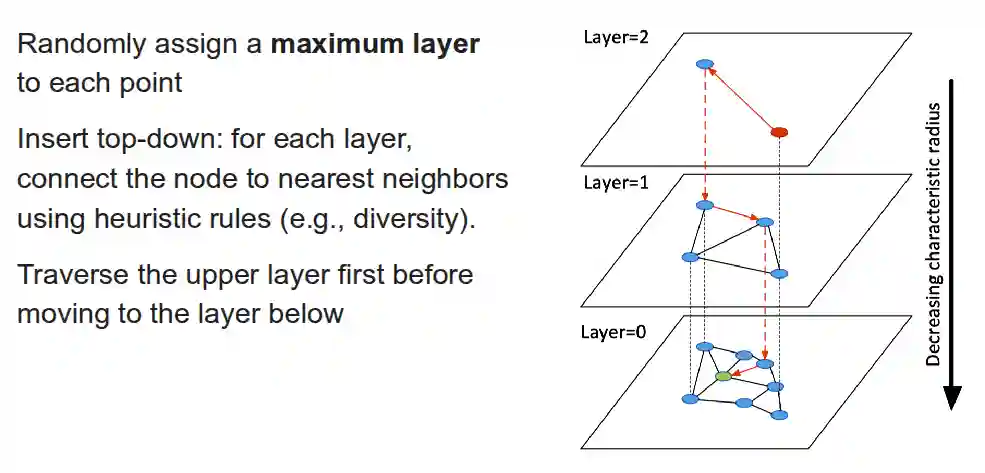
Hierarchical Navigable Small World
- NSW (Navigable Small World)
- Builds a small-world graph where nodes are connected to their close and some faraway neighbors.
- Search is greedy: jump to closer nodes until you can’t get closer.
- HNSW (Hierarchical NSW)
- Adds multiple layers:
- Top layers are sparse (longer-range links).
- Bottom layers are dense (short-range neighbors).
- Search starts at the top layer and drills down layer by layer, refining the search.
References
[1] Pope et al. “Efficiently Scaling Transformer Inference” Curan 2023
[2] Wei et al. “Chain-of-Thought Prompting Elicits Reasoning in Large Language Models” arXiv preprint arXiv:2201.11903 2023
[3] He et al. “PAPI: Exploiting Dynamic Parallelism in Large Language Model Decoding with a Processing-In-Memory-Enabled Computing System” ACM 2025
[4] Dao et al. “FLASHATTENTION: Fast and Memory-Efficient Exact Attention with IO-awareness” Curran Associates Inc. 2022