This note extends the content Markov Processes in this specific context. One nice expansion, which treats the field a little bit more from the behavioural sciences perspectiv eis Intrinsic Motivation and Playfulness.
Standard notions
Explore-exploit dilemma
We have seen something similar also in Active Learning when we tried to model if we wanted to look elsewhere or go for the maximum value we have found. The dilemma under analysis is the explore-exploit dilemma: whether if we should just go for the best solution we have found at the moment, or look for a better one. This also has implications in many other fields, also in normal human life there are a lot of balances in these terms.
In the context of RL, if we exploit too much, we would get a sub-optimal solution. Instead, if we explore too much, we would get a low reward.
Trajectories
Trajectories can be considered our data in RL settings. Intuitively, trajectories are just sequences of states, action and rewards. So: and a trajectory is (the trajectory should be correctly linked, the end state of a single item should be the start state of the other, but this is just a formalism).
Learning the World Model
Given a trajectory, one simple way to estimate transitions and rewards is just the empirical mean:
Which how often we see a sequence in the form where is any reward, in the trajectories, and the are fixed values of interest. Also in this setting, we are using the Markovian assumption (See Markov Chains.
We would also like to learn the rewards
Where are the total numbers of states in the trajectory where the start state is and the action is . Simple as that.
Model-based algorithms
There is something more in the case of simple n-bandit, see N-Bandit Problem. Usually, these kinds of models are more sample efficient. (The model of the world acts acts as some sort of prior). Another positive thing is the online fashion: we can interact with the environment and learn. Model free methods are more suitable to cases where you just need to train and then deploy.
Greedy Approaches
This is a very simple algorithm, it has something in common with the Metropolis Hasting things we have studied in Monte Carlo Methods. We just choose a new action with probability , else, we go for the best solution we have.
Greedy solution
La parte greedy prende solamente l'azione che massimizza il valore atteso per l'azione. Quindi
Il problema è che questo non esplora. Potrebbe trovare il minimo e restare in quello perché la sua stima è quella.
Epsilon greedy solution
La epsilon greedy prova a risolvere questo, tenendo una probabilità di esplorare. Uniform , e con questa probabilità si fa qualcosa random, e in questo modo si aggiorna il resto.
Questo dovrebbe essere l'algoritmo utilizzato per Atari. Problema è che continua ad esplorare anche se ha raggiunto convergenza buona della stima
The key problem of ϵ-greedy is that it explores the state space in an uninformed manner. In other words, it explores ignoring all past experience. It thus does not eliminate clearly sub-optimal actions. From the lecture notes.
Convergence of Greedy
If instead of keeping the sequence of fixed, we make it dependent on the time-step, and assume it satisfies the Robbins-Moro conditions (e.g. with , then it converges to the best solution. This is also why it does very well in practice.
We call Greedy in the limit with infinite exploration, meaning we are assuming we visit a state infinitely often.
Formally this condition is valid if:
- We explore every action pair infinitely often:
- The policy converges to the greedy policy:
Softmax exploration
This is a generalization of the above greedy exploration. We just add a softmax and a temperature parameter that tells how to trade-off between exploration and exploitation:
Algorithm
This is based on (Brafman & Tennenholz ‘02).
This captures the gist of many techniques, but it is more of a theoretical algorithm. We are optimistic at the beginning, then we become more realistic (meaning our assumptions will coincide more with reality after some time).
We have these assumptions: if we don't know we set it to the upper bound set at the beginning. If we don't know , we add another state that gets all the mass: . This is like a black hole state, you will stay there forever, and get a negative or null reward of .
The nice observation is that we don't need to distinguish between exploration and exploitation
The algorithm
Initially we assume that every transition leads to the fairy-tale state, and every reward is the best possible. We just use this temporarily as we know that in the end reality will be different, meaning the actual rewards of the MDP will be lower than the fairy-tale ones.
From the lecture notes:
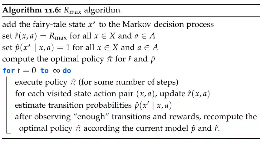
We estimate the reward and transition probabilities as before, using the empirical observations. We need to precisely define the enough, which we will do in the next section.
Bounds on
We use Hoeffding's Inequality, presented in Central Limit Theorem and Law of Large Numbers. And we have:
So we need that amount of actions per state in order to be PAC sure of the reward we have there.
To get an estimate of the value of each state with confidence within an error of . We assume
Then we have another result that tells you that with probability will reach an -optimal policy in a number of steps polynomial to the number of actions, states, times, and then free variables of the above bound. This bounds has some similarities with Provably Approximately Correct Learning.
In the paper, the authors have proved that an optimal policy is reached in polynomial time dependent on the number of states , actions , time, , , and , similar to optimistic Q-learning that we will explore in model-free settings.
Analysis of the Computational Requirements
Memory
We need to keep each state and action in memory. For each state we need to store tuples so the transition probabilities alone are in the order of
Computation Time
We need to apply policy iteration and value iteration each time we have found a new transition probability, which is often costly. The trade-off is the sample-efficiency: these model based models are more efficient on the number of data needed to achieve a good policy, but infer in high computation costs. Furthermore, the update on R max is done at least for each state action pair, so we have at least solutions of the value or policy iteration, which is often quite costly.
Model-free Algorithms
With model free algorithms we don't have access to the underlying state-action-state distributions, thus we cannot do policy evaluation using the Bellman backup as in Markov Processes
Temporal Difference Learning
A Monte Carlo estimate
The idea is to run a trajectory starting from many times and obtaining a Monte Carlo estimate
Where . But the problem in reality is that after have sampled a we cannot go back. So the crude approximation is using a single observation as our approximation, which is . But the variance of the single estimate would be probably quite big, we would like to tamper the problem of this. So we can be more conservative and keep part of the previous estimate. This yields the rule of Temporal Difference Learning for model free value estimation:
In theory we can use a full estimate to approximate the value, but in practice is not possible due to the length of simulation that you would need to do. The expected reward is not available.
Bootstrapping the Value
This is sort of a bootstrap estimate, the idea of using running averages for estimating the value of something. This probably introduces a bias, but I need to investigate this a little bit more. Note that the meaning of Bootstrapping here is different compared to bootstrapping for datasets Ensemble Methods or operative systems.
This Algorithm is called temporal difference as we can write the above value equivalently as:
Where now is now interpretable as a learning rate, and the inside can be seen as a TD error. We can also have here the same convergence bounds that we have used for the epsilon greedy case. This converges to the correct bounds.
This is called On-policy as it can continuously estimate the value function.
Bias Analysis of TD
We have said that bootstrapped samples lead to biased estimates. See https://claude.ai/chat/512eec65-2c84-4871-a973-de90b5757fab.
If is the expected reward at time , an unbiased montecarlo update would be:
If we take the expectation we get:
If we subtract the two, we see that it is unbiased:
Meaning if at step is unbiased, it will remain unbiased at step . This is not true when using bootstrapping as we are assuming the estimate of the next state is noisy.
The gist is: if you start with an unbiased estimate, the monte carlo update will keep it unbiased, bu the Bootstrapped value using TD will not.
Convergence of TD
. The convergence theorem states that if we choose the such that they satisfy the Robbins Moro conditions explained in Active Learning, and we suppose all actions pairs are chosen infinitely often, then the value function converges to the optimal value function, with probability 1. A quite similar convergence argument could be put forward for SARSA.
Gradient Update Interpretation
See RL Function Approximation.
SARSA
On-policy version
We can use TD-learning to do policy evaluation under model-free setting, we now need a way to estimate the best policy without knowing the transitions. Now SARSA comes into play. (now we use instead of for the state because it is more intuitive with the name).
The idea is exactly the same as before, we use bootstrapped samples to evaluate the value:
We now have observed two consecutive couples of states in the trajectory: We can use the same convergence guarantee that we used for TD.
Finding the optimal Policy
After we have estimated these values, we can use the greedy policy
But in practice this method does not explore enough and one needs to do some random exploration, as for the greedy method. In principle, on-policy is more general. This is exactly the bellman optimality condition presented in Markov Processes.
Drawbacks of SARSA
- On-policy nature prevents the reuse of the sampled trajectories. (So one could argue that is not data efficient).
- In practice, the policy does not explore enough.
- This is partially offset by using epsilon exploration.
Off-policy version
If instead of picking the policy via , we can run exactly the same algorithm and get the off-policy version. But now we need to assess the probability having any action. This allows us to estimate it from just a single state, instead of relying on the observed
But this is exactly the same, we are just reweighing the bootstrapped q values following our policy.
Q Learning
The Q-Learning Algorithm
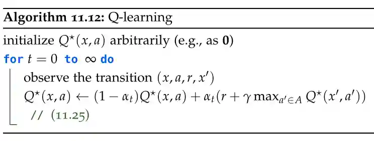 We can interpret the Q-learning algorithm as the analogous of Value Iteration in the model-free case.
The convergence proof is always the same, with Robbins-Moro.
We can interpret the Q-learning algorithm as the analogous of Value Iteration in the model-free case.
The convergence proof is always the same, with Robbins-Moro.
Convergence Bounds of Q-Learning
Compared to [[# Algorithm]], the bounds are tighter: It has been shown that Q-Learning converges to the optimal policy with time polynomial with respect to .
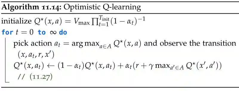
Optimistic Q-Learning
We can use the same idea of in the model-free case. We are optimistic and then, with some time, find better estimates of the values.
Where as we would like to get an upper bound on the best value, not just maximum Reward.
For large Action Spaces Q learning is quite expensive (difficult to find the maximum of all possible actions). This is a common drawback for every tabular-based reinforcement-learning method.
Choosing the bounds
This section briefly argues how the optimistic bounds where chosen: It's easy to see that chosen in this manner effectively upper bounds all possible values:
This bound is already ok for the Optimistic algorithm, the main concept is that the initial value is very very high. In the proof given in the book, one assumes that there is a learning phase where the learning is still showing the optimist behaviour, then it actually starts to learn. But these details are probably irrelevant. The important thing to remember is that we are using the same idea for the algorithm, but here we are model free.
Complexity Analysis
If is the number of states and the number of actions
- Space: We need to store states and actions so the space complexity is ,
- Time: the computation time is just finding the maximum so the complexity is for a single iteration.
In the next section we will try to approximate the state value function, see RL Function Approximation.