Normalizing flows have both latent space and can produce tractable explicit probability distributions (closer to Autoregressive Modelling, they have tractable distributions, but not a latent space). This means we are able to get the likelihoods of a certain sample.
This approach to modelling a flexible distribution is called a normalizing flow because the transformation of a probability distribution through a sequence of mappings is somewhat analogous to the flow of a fluid. From (Bishop & Bishop 2024)
The main idea
The intuition here is that we can both have a latent space and some sort of autoregressive modelling. We want
- An analytical model that is easy to sample from.
- We want this distribution to be able to represent complex data.
- The idea is to use many change of variables,
And you can remember that if we have an invertible matrix $A$ then you can take out the inverse thing.
$$ \begin{align*} p_{x}(x) = p_{z}(A^{-1}x) \lvert \det(A^{-1}) \rvert \\ p_{x}(x) = p_{z}(f^{-1}(x)) \left\lvert \det\left( \frac{ \partial f^{-1}(x) }{ \partial x } \right) \right\rvert = p_{z}(f^{-1}(x)) \left\lvert \det\left( \frac{ \partial f(z) }{ \partial z } \right) \right\rvert^{-1} \\ \end{align*} $$Normalizing Flows
Normalizing flows are direct application of the change of variables formula. we have three desiderata:
- Invertible
- Differentiable
- Preserve dimensionality
The model
$$ f_{\theta}: \mathbb{R}^{d} \to \mathbb{R}^{d}, \text{s.t., } X = f_{\theta}(Z) \cap Z = f_{\theta}^{-1}(X) $$It is important that the transformation is invertible (but this raises also expressivity concerns, because it limits possible functions).
$$ p_{X}(x ; \theta) = p_{z} (f^{-1}_{\theta}(x)) \cdot \left\lvert \det \left( \frac{ \partial f^{-1}_{\theta}(x) }{ \partial x } \right) \right\rvert $$Parameterizing the transformation
We want to find a way to learn the function $f$. The difficulty is having invertible neural networks here, and that it preserves the dimensionality. (Some activations like ReLU are not invertible). And we want to be able to compute the Jacobian efficiently, it is possible to compute it in $O(d)$ if we have a triangular matrix (the determinant is just the diagonal).
$$ x = f(z) = f_{k} \circ f_{k - 1} \circ \ldots \circ f_{1}(z) $$$$ p_{X}(x ; \theta) = p_{Z}(z) \cdot \prod_{i = 1}^{k} \left\lvert \det \left( \frac{ \partial f_{i}^{-1}(x) }{ \partial x } \right) \right\rvert $$Taking the log we have that our final density is:
$$ \log p_{X}(x ; \theta) = \log p_{Z}(f^{-1}(x)) + \sum_{i = 1}^{k} \log \left\lvert \det \left( \frac{ \partial f_{i}^{-1}(x) }{ \partial x } \right) \right\rvert $$And we can do for all points in the dataset. A nice thing about invertibility is:
- We can compute the probability of a true sample
- We can also generate new samples.
The Coupling Layer
The main idea of a normalizing flow is to couple some invertible transformation to be able to get both the likelihood of generated data and the generation itself. Simply stacking linear layers, though invertible, does not work (stack of linear layers is still a linear layer)
Here we use a similar idea present in cryptography for the Feistel network, see Block Ciphers, the idea to partition the space of parameters and apply a transformation to only part of the parameters, this technique has been named real NVP (non-volume preserving). $\beta$ can be an arbitrarily complex function, since it structure allows to preserve that value.
$$ \begin{pmatrix} y_{A} \\ y_{B} \end{pmatrix} = \begin{pmatrix} h(x_{A}, \beta_{\phi}(x_{B}); \theta) \\ x_{B} \end{pmatrix} $$$$ \begin{pmatrix} x_{A} \\ x_{B} \end{pmatrix} = \begin{pmatrix} h^{-1}(y_{A}, \beta_{\phi}(y_{B}); \theta) \\ y_{B} \end{pmatrix} $$$$ h(x_{A}, x_{B}; \theta) = \exp(\theta(x_{A})) \odot x_{B} + \mu(x_{A}, w) $$Where $\odot$ is the element-wise product, and $\mu$ is a function of $x_{A}$ and $w$ (the parameters). You can see that the inverse is quite easy do get.
$$ \frac{\partial y}{\partial x} = \begin{pmatrix} \frac{\partial h}{\partial x_{A}} & \frac{\partial h}{\partial x_{B}} \\ 0 & I \end{pmatrix} $$And this determinant is very easy to compute since it’s a diagonal matrix. This design makes it good!
Training the flow of transformations
$$ \log p_{x}(x) = \log p_{z}(f^{-1}_{\theta}(x)) + \sum_{i=1}^{k} \log \left\lvert \det \left( \frac{ \partial f_{i}^{-1}(x) }{ \partial x } \right) \right\rvert $$And summing for the whole dataset. Because of the structure, we can explicitly evaluate how probable is the sampled sample.
Continuous Normalizing Flows
We don’t know how many layers we would need, the same problem we had in Clustering. We use similar idea of Dirichlet Processes, going into continuous mode, or meta parametrization, and you have continuous normalizing flows, which is something close to (Chen et al. 2019), so that you do not need to set up a specific number of layers. This was the main selling point for these kind of models. Flow matching and diffusion models made them quite famous.
Resolution is quite slow because it preserves dimensions (a lot of computational time).
Planar Normalizing Flows
Given a latent variable $z \in \mathbb{R}^{d}$ and $x \in \mathbb{R}^{d}$ the mapping is a function in the form:
$$ x = f(z) = z + u \cdot h (w^{T}z + b) $$Where $f$ is continuously differentiable and $h(\cdot)$ is a non-linear activation others are learnable parameters.
$$ p_{z}(z) = \prod_{i} \frac{1}{\sqrt{ 2\pi }} \exp(-z^{2}_{i} / 2) $$Then one can prove that the arg min of this model has the form:
$$ \begin{align*} \arg \min \mathcal{L} &= \arg \max \log p_{x}(x) \\ &= \arg \max \log p_{z}(z) + \log \lvert \det(J^{-1}) \rvert \\ &= \arg \max \log - \lvert z \rvert ^{2} / 2 - \log \lvert 1 + h'^{T}u^{T}w \rvert + \text{ constant} \end{align*} $$Where we have substituted the definition of the Gaussian latent seen that the Jacobian is:
$$ J = \frac{\partial x}{\partial z} = I + h' \cdot u^{T}w $$The Architecture
Squeeze
We want to reshape from $4 \times 4 \times 1$ to $2 \times 2\times 4$ dimensionality thing. One drawback is that at each coupling layer we process only half of the data, shuffling helps plain the processing. Using usually some checked structure to split it into many parts so that we can use flow in parallel So they just change the spatial resolution of the layers.
Flow step
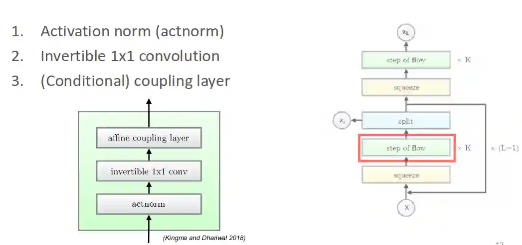
Act norm is for example a batch norm see section in Convolutional Neural Network.
1x1 Convolutions
1x1 convolutions are generalizations of permutations (i.e. they contain permutations, if the matrix is a permutation matrix), introduced in (Kingma & Dhariwal 2018).
$$ W = PL(U + \text{diag}(s)) $$Where $L$ is lower triangular, $P$ is a permutation matrix, and $U$ is upper triangular (with 0 on diagonal). One can observe that the log determinant of this matrix is just the sum of $s$, which is quite quick to compute. The log determinant of this matrix would just be $\sum s_{i}$ because of the above properties.
$$ \begin{pmatrix} y_{A} \\ y_{B} \end{pmatrix} = \begin{pmatrix} h(x_{A}, \beta(x_{B}, W)) \\ x_{B} \end{pmatrix} $$Small History of Early Flows
- NICE (Dinh et al. 2015), Nice, introduces a first working version for NF, but just does swapping for the variables, not quite efficient, and uses additive coupling layer.
- RealNVP (Dinh et al. 2017): introduces affine coupling layer (adds scale) and a checkboard pattern to better mix the values.
- GLOW: (Kingma & Dhariwal 2018): adds the invertible 1x1 convolutions, first paper that generates something high quality, community now sees NFs as architectures that could actually work.
Applications
Common applications are:
- Super-resolution
- You learn a distribution of possible super resoluted images.
- Disentanglement of fetures (akin to what they do in stylegans, see Generative Adversarial Networks).
- Multimodal modeling (related to 3D vision applications).
- 3D shape modelling (see Parametric Human Body Models).
- 3D pose estimation
SRFlow
Paper -> (Lugmayr et al. 2020). SRFlow modifies the beta by conditioning on the higher resolution image, achieving a super resolution with flow methods. Since it needs to keep the resolution, the input is conditioned in the beta layer. after n encoding step.

Architecture from the paper.
We have and encoder $u = g_{\theta}(x)$ that maps the low resolution image to $u$, then activation maps are modulated with this $u$ value, in a manner somewhat similar to StyleGANs, with feature modulation.
Forward: $h^{n+1} = \exp(\beta^{n}_{\theta, s}(u)) \cdot h^{n} + \beta_{\theta, b}(u)$ Inverse: $h^{n} = (h^{n+1} - \beta_{\theta, b}(u)) \odot \exp(-\beta^{n}_{\theta, s}(u))$ Log determinant is: $\sum \beta^{n}_{\theta,s}(u)$
The encoding of the features, is somewhat similar to what they do in Log Linear Models. After training, we can have multiple variants of the same image, in plausible versions.
StyleFlow
This is the paper -> (Abdal et al. 2021). Other works are for example StyleFlow, extension of styleGAN, described in Generative Adversarial Networks, where you can interpolate between identities, or make other continuous disentangled modifications.
They use Normalizing Flows to create encoded weights of the style (conditioned with some attribute, e.g. lighting, head pose etc). You can control some nice features such as:
- Head pose
- Lighting
What they mainly do is changing the mapping between the latent space to the mapped features that they then feed into the synthesis model. They found that the $W$ space of the style features where highly expressive, we want to control the features of this space so that we can better choose exactly the shapes that you need. They use attribute conditioned continuous normalized flows.
- Generate synthetic data, and collect pairs of latent styles and images. They use a pretrained GAN model to do this part. Probably thousands of samples.
- From the images, they estimate a set of attributes (light, pose etc.)
- They use the attributes to condition the NF to generate the latent styles. And they use it for many many blocks.

Image from the paper | Conditional continuous normalizing flow (CNF) function block realized as a neural network block. Note that the learned function, conditioned on attribute vector at , can be used for both forward and backward inference.
The difference is that we have time input since it is a continuous normalizing flow. You can reverse back, change features and forward to change some features of the face, which is quite cool.
C-Flow for multi-modal data
The idea here is to condition one flow with another flow, and use it for more complex part. This section needs further study, because I did not understand.
Here they introduce the translation between image and point cloud, flow A conditioning, flow B the flow to be conditioned.

Image from the paper | The two flows can work in different modes of data, but in this way they can share some, not well defined, information
In the paper they show results for style transfers in shows. It needs a lot of compute for low resolution (which is the main problem for normalizing flows). And usually they are not so high dimensional.
Other applications
Pose estimation: You have some poses, and you can find the probability of some poses (so you can take just the highest probability pose in a maximum likelihood fashion).
PointFlow: From Gaussian point cloud to chairs and similar stuff.
References
[1] Dinh et al. “Density Estimation Using Real NVP” arXiv preprint arXiv:1605.08803 2017
[2] Lugmayr et al. “SRFlow: Learning the Super-Resolution Space with Normalizing Flow” ECCV 2020
[3] Abdal et al. “StyleFlow: Attribute-conditioned Exploration of StyleGAN-Generated Images Using Conditional Continuous Normalizing Flows” ACM Trans. Graph. Vol. 40(3), pp. 21:1--21:21 2021
[4] Dinh et al. “NICE: Non-linear Independent Components Estimation” arXiv preprint arXiv:1410.8516 2015
[5] Chen et al. “Neural Ordinary Differential Equations” arXiv preprint arXiv:1806.07366 2019
[6] Kingma & Dhariwal “Glow: Generative Flow with Invertible 1x1 Convolutions” arXiv preprint arXiv:1807.03039 2018
[7] Bishop & Bishop “Deep Learning: Foundations and Concepts” Springer International Publishing 2024